Previous | Table of Contents | Next

2.

Settlement Pattern, Site Typology, and Demographic Analyses: The Anasazi, Archaic, and Unknown Sites

Lynne Sebastian and Jeffrey H. Altschul

¶ 1    This chapter presents analyses of the site data collected during the inventory survey. The data are summarized, the site typology used during the survey is evaluated, and settlement pattern and demographic analyses of the data are reported. The 957 sites recorded by the project contained 730 Anasazi components, 9 Archaic components, and 344 components of unknown cultural affiliation. Most of this report concerns the Anasazi components; the Archaic and Unknown components will be discussed in separate sections at the end of the chapter.

¶ 2   The basic data used in the analyses reported here are presented in two electronic appendices. Appendix 2.1 presents information on the components identified at each site and the features present in those components, along with subsidiary information on component and feature sizes and temporal affiliation of each component. Each line in Appendix 2.1 represents a single feature within a component at a site. Appendix 2.2 contains summary data on the artifact assemblage recorded for each component. Each data line in Appendix 2.2 represents a summary of all artifacts affiliated with a single component at a site.

¶ 3   The research reported here was designed to address six major goals. The first goal was to identify temporal/functional components at the sites recorded during the survey. The second was to code and computerize the survey data in such a way that the artifacts from each site could be assigned to those components and so that artifact, feature, and component data could be computer manipulated. The third goal was to evaluate spatial and temporal patterning in the component, feature, and artifact data. The fourth goal was to evaluate the site typology used to organize the survey data, to assess its effectiveness and consider its functional implications. The fifth goal was to examine the Anasazi settlement pattern in terms of correlations between components of different types and variables of the natural and social environments. And the sixth goal was to examine the demographic implications of the site and artifact data recorded during the survey.

¶ 4   The first major section of this chapter describes the procedures used to computerize the site survey data and the methods employed in the typology, settlement pattern, and demographic analyses. Subsequent sections present a summary discussion of the data base, the site typology evaluation, the settlement pattern and demographic analyses, and the discussions of the Archaic and Unknown components.

Computerization of the Survey Data

¶ 5   The first step in the survey analysis was to code the site form data on structures and features in such a way that they could be subjected to computer analysis. Because the data were collected largely in a narrative and cartographic format rather than in a format designed for direct computerization, this required that many judgments be made. The resultant computer data must be considered to be somewhat subjective, because bias could have been introduced by the analysts during the coding process. On the other hand, all of the coding was done by one individual (the senior author), so any introduced biases should be consistent from area to area.

¶ 6   The information used to create the computer data base was taken from the Site Description section on pages 4 and 5 of the site form (see Appendix 1.1) and from the site map appended to the site form. In cases where there was a discrepancy between the site description and the map, information from the “Additional description of site features” portion of the site form was used in an attempt to resolve the differences. If questions remained, the project director and survey crew chiefs were consulted.

¶ 7   The variables recorded in the computer data base are listed in Table 2.1. Area, county, and culture were taken from the first page of the survey form. There was some variability in the criteria used by the survey crew to assign sites to the Anasazi and Unknown culture categories. For the purposes of the computer data base, any component that contained fewer than five ceramic sherds and could not be definitely assigned to the Archaic, Anasazi, or Navajo culture categories on the basis of diagnostic artifacts or features was classified as Unknown. Components containing more than five Anasazi sherds and not definitely assignable to the Archaic or Navajo culture categories were classified as Anasazi.

Table 2.1. Variables recorded in computerized data base.
Variable
Area
County
Culture
Component Number
Component Type
Component Size
Date Group
Feature Type
Feature Number
Feature Area
Mound Height
Number of Visible Rooms
Number of Estimated Rooms

¶ 8   During the computer coding phase of the research, both temporal and functional criteria were used in defining components on the sites recorded during the survey. Temporal components were identified on the basis of ceramic dates assigned to features at the site; all features assigned to the same date group (Table 2.2; refer to ceramics, chapter 4 for a discussion of the derivation of these groups) were considered to be part of the same temporal component. Features containing ceramics from more than one date group were assigned to hybrid date groups—e.g., features containing ceramics dating to both Date Group (DG) 300 (A.D. 890 to 1025) and DG 400 (A.D. 1030 to 1130) were assigned a 350 date group (A.D. 890 to 1130); features containing ceramics dating to DG 200 (A.D. 700 to 880), DG 300 (A.D. 890 to 1025), and DG 400 (A.D. 1030 to 1130) were assigned a 234 date group (A.D. 700 to 1130). Features for which no ceramic dates could be determined or from which no ceramics were recovered were assigned to a date group of 999 (unknown) unless they were physically surrounded by and functionally compatible with dated features. In the latter case the undated features were considered to be part of the same temporal component as the nearby dated features.

Table 2.2. Ceramic date groups used in identifying temporal components.
Date Group	Dates (A.D.)	Included Date Group
100	550-750	-
150	550-880	100, 200
123	550-1025	100, 200, 300
200	700-880	-
250	700-1025	200, 300
234	700-1130	200, 300, 400
300	890-1025	-
350	890-1130	300, 400
345	890-1230	300, 400, 500
400	1030-1130	-
450	1030-1230	400, 500
500	1130-1230	-
999	Unknown	-

¶ 9   Functional component types were assigned, as much as possible, on the basis of the site type designations given to each site by the survey crews. There were two main instances in which this was not done. The first concerned the “fieldhouse” designation. During the survey, there was some variability from area to area in how this designation was applied. In Kin Klizhin, for example, only those sites containing definite evidence of a structure—foundation alignments, etc.—were classed as fieldhouses. In Kin Bineola, on the other hand, sites consisting of an artifact scatter containing a concentration or even a scattering of rubble elements were often classified as fieldhouses. To increase consistency and to preserve a distinction that we felt would be functionally important, in this report we classify only those components that contained actual indications of a structure as fieldhouses. Most of the reclassified components were assigned to one of the two scatters with feature component types discussed below.

¶ 10   The second major deviation from the survey functional classifications concerned those artifact scatters that incorporated rock elements. In cases where sites consisting of artifact scatters and slabs or other unburned rubble were not classified as fieldhouses during the survey, they were recorded as two different site types: one artifact scatter and one slab/fire-cracked rock concentration. Because we believed that the artifacts and the rock features were most likely to be related parts of a single component rather than two functionally distinct components, we created a new component type: artifact scatter with slabs. A similar situation arose with sites consisting of an artifact scatter and a hearth or a concentration of burned elements. The survey had also classed these features as two distinct components: a scatter and a slab/firecracked rock concentration. We classified them as another new functional type: artifact scatter with hearth, the hearth term being used to cover all evidence of burning—actual hearths as well as firecracked rock and burned slabs. Table 2.3 lists the functional component types used in creating the computer data base.

Table 2.3. Functional component types used in the computer database.
Component Type
Habitation
Fieldhouse
Ledgeroom(s)
Sherd scatter
Sherd/lithic scatter
Hearth(s)
Baking pit(s)
Water control
Cist/storage
Shrine
Fieldhouse/water control
Chacoan structure
Lithic scatter
Road segment/trail
Great kiva
Rock art
Stairs
Artifact Scatter with slabs
Artifact Scatter with hearth
Road-associated (e.g., herradura)
Building stone quarry
Other
Unknown
Unknown prehistoric

¶ 11   Each temporal or functional component at a site was assigned first a unique, sequential component number (1 through n for each site) and then a component type. On sites where more than one cultural category was represented, the unique, sequential numbering system was maintained. On a site with two Anasazi components and an Unknown component, for example, the Anasazi components would be numbered 1 and 2, while the Unknown component would be numbered 3, even though it was the first Unknown component at the site. Finally, the size of each component was coded, either from information on page 4 of the survey form or by measuring the extent of the component as depicted on the survey map. Once the components had been identified, all of the features within each component were coded individually. Each feature was first assigned a feature type (Table 2.4). Generally the types were those assigned by the survey crews, but in cases where the survey site map showed hybrid types (cist/hearth) a decision had to be made based on the field notes. We felt that the distinctions between “pithouse” and “possible pithouse” and between “kiva” and “possible kiva” as made by the survey crews were potentially important, so we created new feature types for the two “possible” categories. We also added the feature types trash mound, plaza, rock alignment, circular masonry structure, possible room/ramada, burial slab scatter, and isolated room, based on frequently encountered notations on the site forms and maps.

Table 2.4. Feature types used in the computer database.
Feature Type
Roomblock
Fieldhouse
Ledgeroom
Sherd scatter
Sherd/lithic scatter
Lithic scatter
Hearth
Baking pit
Cist
Storage room
Shrine
Great kiva
Chacoan structure
Road
Trail
Rock art
Stairs
Slab/fire-cracked rock scatter
Kiva
Fieldhouse/water control
Lithic concentration
Pot drop
Unknown structure
Unknown feature
Canal/ditch
Dam
Check dam
Cairn
Oven
Quarry
Burial
Ramada/lean-to
General site scatter
Pithouse
Stone circle
Water control (unspecific)
Rockshelter
Trash mound
Possible pitstructure
Plaza
Possible kiva
Rock alignment
Circular masonry structure (herradura?)
Possible room (ramada?)
Burial slab scatter
Isolated room

¶ 12   Each feature was then assigned a feature number that was sequential within each feature type (hearth 1 through n, roomblock 1 through n, etc.), within each component. Where feature numbers had been assigned in the field we retained them if possible; when sites were divided into temporal or functional components this was not always possible, however. If the survey crews had not assigned feature numbers in the field, which was usually the case with smaller features such as hearths, then numbers were assigned during coding and recorded on the survey field maps for future reference.

¶ 13   Features that constituted the entire component were not coded separately if the component and the feature were of the same type. For example, a component of type baking pit that consisted of a single feature of type baking pit and nothing else would not have the baking pit coded as a separate feature. If the component type and feature type differed—e.g., a component of type water control consisting of a feature of type check dam—then the feature was coded.

¶ 14   Feature type and number were coded for all features within a component; the last four variables in Table 2.1—feature area, mound height, visible rooms, and estimated rooms—were coded for only selected feature types. Feature area was coded for all structures, both above-ground and subterranean, and for trash mounds and scatters. Mound height was recorded for above-ground structures and for trash mounds. Room counts were recorded for Chacoan structures, roomblocks, fieldhouses, and ledgerooms; estimated rooms includes both visible rooms and estimated additional rooms.

¶ 15   Once the survey data had been coded, we attempted to match the artifacts with the newly defined components. This proved to be a difficult task, because the unit of analysis for the artifacts was the feature, and many features were not numbered in the field or had to be renumbered once the components were defined. During computer coding of the artifact data, component codes were assigned, but these components were defined on the basis of depositional environment and were intended to provide information concerning depositional history of the sites. Because these components were not intended to be functional or temporal units, the artifact component codes could not be used as the basis for the settlement pattern and site typology analyses. There are undoubtedly some errors in the matching of temporal/functional components and artifact assemblages contained in Appendix 2.2, but the codings that produced these artifact summaries were done by a single individual, so the summaries should be at least internally consistent.

Summary of the Site Survey Data

¶ 16   This section of Chapter 2 presents summary data characterizing the Anasazi components recorded during the survey. Most of this information has to do with the component/feature data presented in Appendix 2.1; the summary of the artifact data from Appendix 2.2 is less detailed because the various artifact classes are discussed at length in other reports. The major axes of variability along which the data are characterized are: a) differences among the four survey areas, b) differences among the component types, and c) differences among the temporal periods. A series of maps showing the distribution of components of different types were prepared, and a collection of tables were generated using the SAS software package (Ray 1982) on an IBM 360 computer to summarize these data.

¶ 17   In a subsequent section of this chapter we will present a detailed evaluation of the site typology (and to some extent of the feature typology) used during the survey. For the purposes of the data summaries presented here, we accepted the survey typology at face value and used it to order the data. In the typology evaluation section, information from these summaries will be used in conjunction with other data and with computer analysis techniques to assess the functional content and appropriateness of the typology.

¶ 18   In general, the typology was found to be quite successful although a number of suggestions for further refinements are offered. One important observation about the typology should be made before the data summaries are presented. Even though the functional content of the site/component type names varies in specificity (e.g., function-based terms such as “fieldhouse” versus descriptive terms such as “ceramic scatter”), the criteria used for assigning sites to these types were strictly morphological. Therefore this is a morphological typology based on generally objective attributes. The suitability of the suggested functional classifications for the various site/component types will be assessed in the Functional Implications section below.

Characterization of the Component Types

¶ 19   The first step in characterizing the site data was to determine how many components there were of each type. As Table 2.5 shows, the most common component type was habitation, which constitute more than 18 percent of the sample. This pattern occurs despite the low proportion of habitation sites in the Chacra Mesa survey area; in the other three survey areas habitations constitute over 23 percent of the components. The second most common component type is the artifact scatter with hearth category. The other most common component types are fieldhouses, rock art panels, and baking pit sites. The basic component type data were also characterized according to spatial and temporal variability, topics that are discussed in separate sections below, and according to mean size. Table 2.6 provides data on mean sizes for the component types for which such data are appropriate. The general characteristics of the various component types in terms of kinds and numbers of features are discussed individually below.

Table 2.5. Component type proportions within each survey area.

Table 2.6. Mean component size data.
Component Type	Mean Size m2
Habitation	13,934.3
Fieldhouse	4,332.7
Ledgeroom	3,144.4
Sherd scatter	4,300.4
Ceramic and lithic scatter	2,007.3
Hearth	5,112.2
Baking pit	14,786.0
Water control	2,473.2
Cist/storage	316.6
Shrine	1,871.9
Great kiva	672.2
Chacoan structure	15,842.3
Scatter with slabs	2,605.6
Scatter with hearth	7,549.4

¶ 20   Habitation components include sites with pithouses, sites with above-ground roomblocks, and sites with both types of residential structures. Of the 133 habitation components, 34 have only pitstructures, 55 have only roomblocks, and 44 have both; spatial and temporal patterning in these different types of structures are discussed in a later section of this chapter. The roomblock components contain an average of 1.12 roomblocks; the components with both roomblocks and pithouses contain an average of 1.14 roomblock features. The mean number of visible rooms in all roomblock features is 3.1; the mean number of total estimated rooms is 7.0. The roomblock sites contain an average of 0.9 kivas and possible kivas. The roomblock/pithouse components have an average of 0.3 kivas and possible kivas per component.

¶ 21   The pithouse components contain an average of 1.7 pithouses and 3.2 possible additional pithouses. These figures are strongly affected by the presence of Shabik’eshchee Village in the sample, however, because this one site contains 18 pithouses and 49 possible pithouses. If this site is excluded from the sample, the other pithouse sites contain an average of 1.1 pithouses and 1.8 possible pithouses. The components that include both forms of residential structures contain an average of 0.2 pithouses and 1.6 possible pithouses.

¶ 22   Two other common features found on the habitation components are trash mounds (n=37 among all 133 habitation components) and trash scatters (n=61). All of the trash mounds are on the roomblock and roomblock/pithouse components; the definable trash concentrations occur on approximately half of the components in all three habitation subtypes.

¶ 23   Baking pits are common on pithouse components (n=33 on the 34 pithouse components) and less so on roomblock and roomblock/pithouse components (n=25 among 99 components). The same pattern occurs for cist/storage features; n=58 for 34 pithouse components, and n=22 for the 99 roomblock and roomblock/pithouse components. The presence of Shabik’eshchee Village in the sample also affects this latter result strongly, however. This site contains 33 of the 58 cist/storage features recorded for pithouse components. Concentrations of slabs and/or fire-cracked rock are also common on habitation components, especially the pithouse only components (n=43 for pithouse components; n=41 for roomblock and roomblock/pithouse components).

¶ 24   Site layout for habitations (Figure 2.1a, b, c) tends to be quite consistent over time and across space. The pithouse villages exhibit no formal patterning, and their structure appears to be largely a function of the local terrain. At many sites, close proximity of the pithouse depressions suggests that they represent successive rather than contemporaneous occupations. Both combined pithouse/roomblock and roomblock-only components tend to have a northwest/southeast orientation, with occasional west to east orientation. Roomblocks tend to lie in an arc or line trending northeast/southwest along the northwest edge of the site, with any pitstructures (both pithouses and kivas) located immediately to the southeast. Formal midden deposits, where they occur, generally are located to the east/southeast of the pitstructures. Informal trash deposits often are located in the same position, but tend to be somewhat more variable in their location. Baking pits, hearths, and other extramural features are scattered about the sites and do not exhibit any particular patterning other than a tendency not to occur “behind” (to the northwest of) the roomblocks on sites that have them.

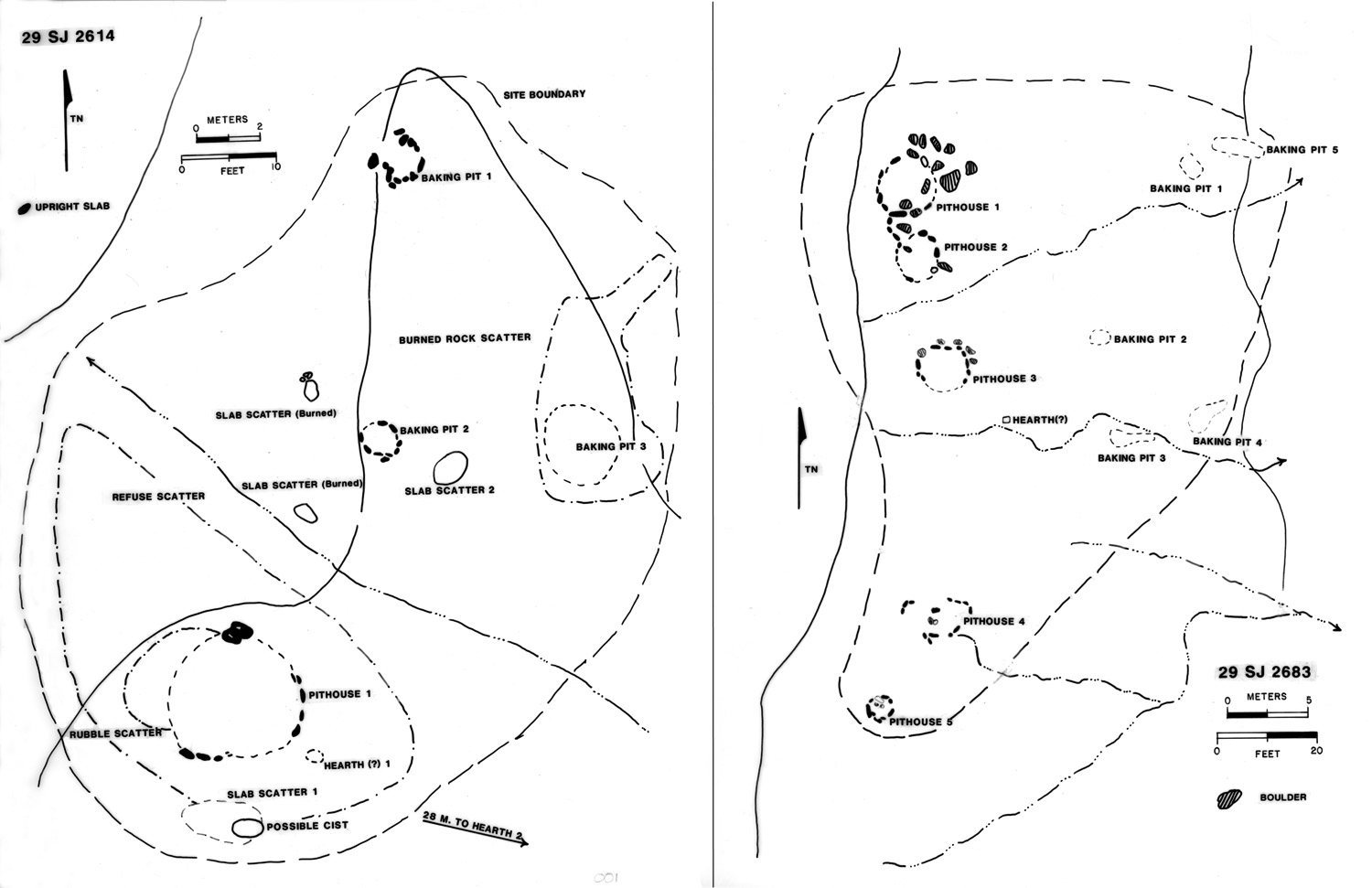Figure 2.1a. Examples of habitation component layouts: 29SJ 2614, A.D. 500-750 (DG 100) and 29SJ 2683, A.D. 550-750 (DG 100).

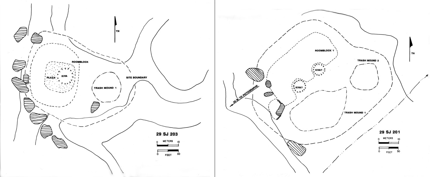Figure 2.1b. Examples of habitation component layouts: 29SJ 203, A.D. 1030-1130 (DG 400) and 29SJ 201, A.D. 1030-1130 (DG 400).

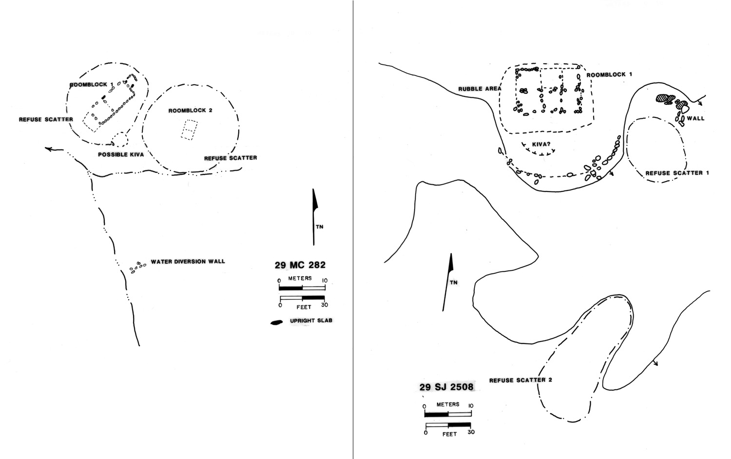Figure 2.1c. Examples of habitation component layouts: 29SJ 282, A.D. 550-750 (DG 100) and 29SJ 2508, A.D. 1030-1130 (DG 400).

¶ 25   Fieldhouse components (n=72) contain an average of 1.1 fieldhouse structures (mean visible rooms=1.1 per fieldhouse, mean estimated rooms=1.4 per fieldhouse). The most common feature on these components aside from the fieldhouse structures themselves are slab/fire-cracked rock concentrations (n=39 among the 72 components). Other commonly noted features are discrete trash concentrations (n=18), baking pits (n=12), and cists (n=10). As these numbers indicate, the average number of features of all types per fieldhouse component is low—2.8 features per component—compared with the number of features on habitation components—6.7 features per component.

¶ 26   Fieldhouse components exhibit three general site plans (Figure 2.2a, b, c). By far the most common type consists of a rubble concentration with a few alignments or upright slabs marking the base of the room or rooms of the fieldhouse surrounded by a light, diffuse artifact scatter. Occasionally hearths or other extramural features occur on these components, but in general they are rare. These components show no particular orientation, but they do tend to occur on the ends of low ridges on the floodplain.

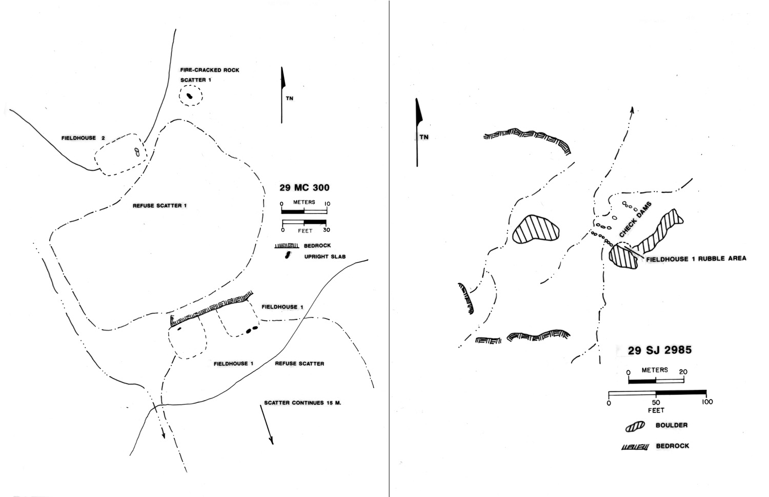Figure 2.2a. Examples of fieldhouse component layouts: 29Mc 300, A.D. 890-1025 (DG 300) and A.D. 1030-1130 (DG 400); and 29SJ 2985, A.D. 1130-1230 (DG 500).

Figure 2.2b. Examples of fieldhouse component layouts: 29SJ 2791, A.D. 890-1025 (DG 300) and 29Mc 250, A.D. 1130-1230 (DG 500).

Figure 2.2c. Examples of fieldhouse component layouts: 29SJ 207, A.D. 1030-1130 (DG 400) and 29SJ 324, A.D. 890-1025 (DG 300).

¶ 27   The second common plan of fieldhouse components consists of multiple fieldhouses, each with its own associated artifact scatter and, on occasion, extramural features. These components probably represent multiple but functionally similar uses of particularly favorable locations.

¶ 28   The third general site plan for fieldhouses consists of one or more fieldhouse structures, associated artifact scatters, and a number of extramural features, often scattered over a large area. The most common features on these sites are baking pits and burned rock concentrations, but associated water-control features also occur. Without excavation data it is impossible to determine whether these sites represent fieldhouses that were occupied over a longer period or more intensively than those on the other sites or whether these components represent palimpsests of multiple, functionally differentiated occupations that could not be separated on the basis of survey data.

¶ 29   Ledgeroom components (n=36) contain an average of 1.7 ledgeroom structures per component; mean visible rooms per ledgeroom structure is 1.3, mean estimated rooms per structure is 1.4. Other common features on ledgeroom components are hearths (n=15) and baking pits (n=9). The ledgeroom components have a slightly higher number of features than fieldhouses (average=3.1) features per component).

¶ 30   As the mean room number data show, multiroomed ledgerooms are relatively rare, but so are single isolated ledgerooms. Most often these components consist of a series of separate single-room structures built along a rock face or in adjacent small shelters (Figure 2.3a, b, c). There is a slight tendency for these components to face east or southeast, but west- and south-facing structures are common, and two ledgerooms have a partially northerly exposure. In general, it appears that these components were located to take advantage of sheltered locations with only minimal attention to direction of exposure.

Figure 2.3a. Examples of ledgeroom component layouts: 29SJ 293, A.D. 1030-1130 (DG 400) and 29Mc 290, A.D. 1030-1130 (DG 400).

Figure 2.3b. Examples of ledgeroom component layouts: 29Mc 217, A.D. 1030-1130 (DG 400) and 29Mc 255, A.D. 890-1025 (DG 300).

Figure 2.3c. Examples of ledgeroom component layouts: 29SJ 2742, unknown date (DG 999) and 29 Mc 295, A.D. 1030-1130 (DG 400) and A.D. 1130-1230 (DG 500).

¶ 31   Most of the sherd scatter components (41 out of a total of 50 components) had no features. The most common feature on the other nine components was trail segments (n=4). Likewise, most of the sherd and lithic scatter components (28 of the 34 components) contained no features. Interestingly, no trail segments were recorded on these sites; rock scatters and sherd concentrations were the most common features.

¶ 32   The hearth components (n=16) consisted either of a single hearth feature (n=4) or of a combination of hearths and fire-cracked rock concentrations. Those components with more than one thermal feature contain an average of 2.7 features per component. The baking pit components (n=69) occasionally consisted of a single feature (n=6), but generally contained multiple features (121 baking pits on the 63 multiple feature components). Other common features on these sites are burned rock scatters (n=85) and hearths (n=19); at least some of the former probably represent additional baking pit features.

¶ 33   The 30 water control components consist of 27 check dams, 4 other dams, 8 canal/ditch features, and 10 other water control features of unknown type. The 18 cist/storage components include 3 isolated cist/storage features, 9 other cists, and 13 storage rooms. Three of the nine shrine components consist of single isolated shrine features; seven other shrines and one kiva with an enclosed plaza (29Mc 292) in the Kin Bineola area) are among the other features recorded on the remaining shrine components.

¶ 34   The artifact scatter with slabs (n=44) and artifact scatter with hearth(s) (n=89) components are dominated by slab/fire-cracked rock concentrations (n=218 for both types combined). The other common feature types on these components are hearths (n=49), which of course occur only on scatters with hearth components, and baking pits (n=22), although storage cists, discrete trash concentrations, and other features also occur.

¶ 35   Two great kiva components and five Chacoan structure components were recorded. The two great kiva components are an isolated structure on Chacra Mesa with a trash mound and three possible rooms in association (site 29SJ 2557; Figure 2.4) and a great kiva in association with two roomblocks and a trashmound in the Kin Bineola area (site 29Mc 261; Figure 2.5).

Figure 2.4. 29SJ 2557. Isolated great kiva on Chacra Mesa.

Figure 2.5. 29Mc 261. Great kiva and associated features in Kin Bineola community.

¶ 36   The Chacra Mesa great kiva component is the latest component of this type in the survey sample. Based on surface ceramics it was dated between A.D. 1075-122511 [CLOSE]Beginning and ending occupation dates were established for each feature based on assessment of the beginning and ending production dates of the ceramic types in an assemblage. These begin and end dates, which were used in the cluster analysis to establish the date groups (see Chapter 4) were not used for analytical purposes. However, some readers may find these “raw” dates of interest, particularly for prominent site types such as Chacoan structures and great kivas. and was placed in the A.D. 1130 to 1230 (DG 500) date group by the cluster analysis. Not only is it an isolated component in the sense of having no other components as part of the same site, there are no other contemporary components of any kind near it. It is, however, located in the northeast part of the study area where most of the habitation sites of all time periods are located. The Kin Bineola great kiva component is contemporaneous with the other features on the site: two roomblocks, each containing perhaps 8-10 rooms, and a trashmound 37 by 16 meters by 50 centimeters high. The great kiva itself is 10-11 meters in diameter and surrounded by a number of small rooms (visible rooms=13; estimated rooms=17). All features at this site yielded ceramics dating to A.D. 750 to 1000 (DG 250). This is the only case from this survey of a great kiva being found in association with a village site rather than a Chacoan structure; it is also the earliest great kiva found by the survey.

¶ 37   The Kin Klizhin great house (29SJ 1413; LA 4975; Figures 2.6 and 2.7a, b, c) is a small but imposing structure located on a sandy knoll above Kin Klizhin Wash. The great house has attracted archeological attention for over a century (e.g., Morrison 1876, Boone 1939; Hewett 1905; Holsinger 1901; Judd 1954:57; Marshall et al. 1979:69-72; Vivian 1970). The structure dates from the late eleventh century; tree-ring dates from unprovenienced samples collected by Hawley in 1932 are reported in Bannister et al. (1970:24): 1038p-1086++v, 1065p-1087c, and 1066p-1087c. Based on surface ceramics identified by the survey, Kin Klizhin was dated to A.D. 1050-1175 and was assigned to the A.D. 1030-1130 (DG 400) date group by the cluster analysis. The 40 by 50 meter, two to three story great house contains 13 visible and 20 estimated rooms. There are two visible enclosed kivas and a third, tower kiva with standing walls 5-6 meters above the 3 meter high rubble mound. Walls are constructed of banded core-and-veneer masonry. East of the structure, discontinuous segments of a low, semi-circular wall connect to the north and south ends of the roomblock to form a large plaza area To the north of the plaza is a scatter of diffuse refuse. A low, dune obscured trashmound lies to the southeast of the great house; a possible road segment was also noted in this area of the site. The structure is described in greater detail in Marshall et al. (1979:69-72).

Figure 2.6. Kin Klizhin Chacoan structure (29SJ 1413; LA 4975) plan view.

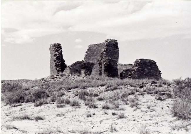Figure 2.7a. Kin Klizhin Chacoan structure looking southwest.

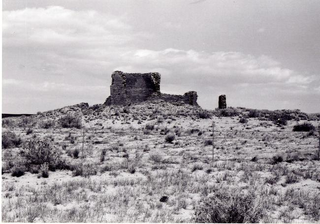Figure 2.7b. Kin Klizhin Chacoan structure looking west.

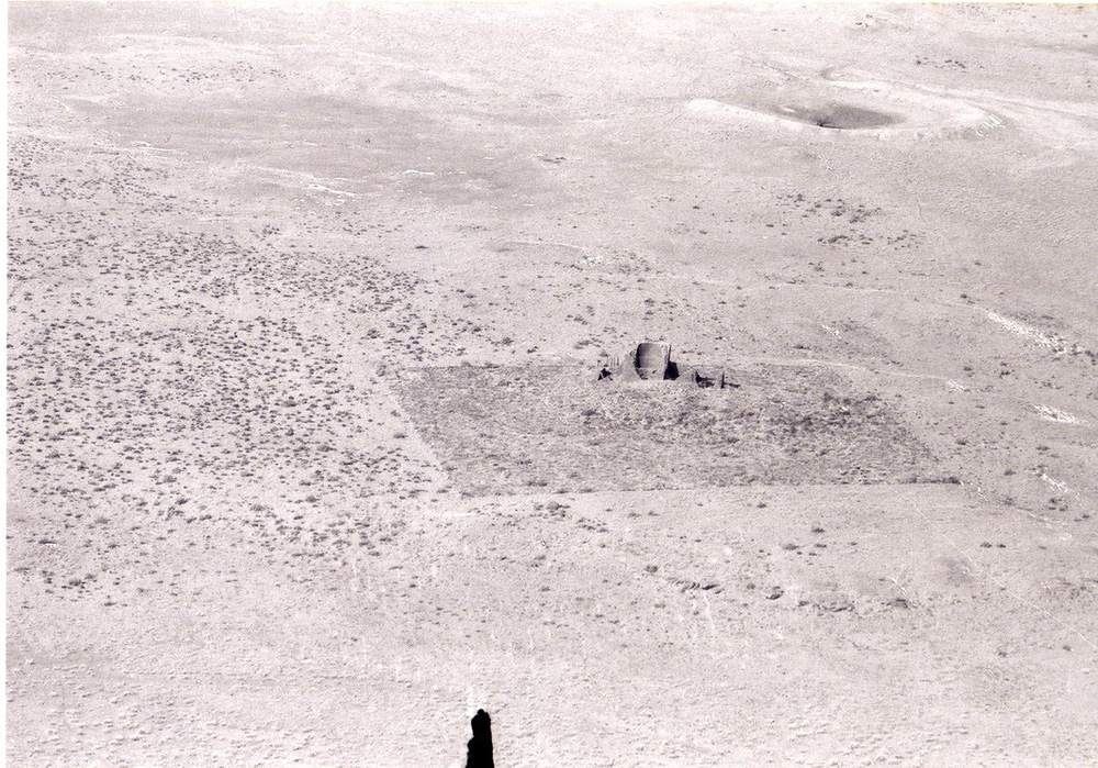Figure 2.7c. Aerial view of Kin Klizhin Chacoan structure looking west.

¶ 38   Three Chacoan structure components were recorded for the Kin Bineola study area, but one of these (site 29SJ 2531) is a trashmound with associated features that is almost certainly part of the Kin Bineola outlier site (29SJ 1580; LA 18705); this component will be described as part of that site below. The Kin Bineola great house (Figures 2.8 and 2.9) is located on open terrain which faces the southeast. Like Kin Klizhin, Kin Bineola has been a focus of archeological interest since the late nineteenth century (e.g., Hewett 1905; Holsinger 1901; Judd 1954; Kluckhohn 1967; Lyons and Barde 1972; Marshall et al. 1979:57-68; Vivian 1970). The massive, E-shaped structure opens to the south-southeast and measures approximately 106 meters east/west by 46 meters north/south. The structure once rose to a height of three stories, and as a result, the collapsed masonry forms a substantial rubble mound. Marshall et al. (1979:58) estimated that 105 ground floor rooms, 58 second floor rooms, and 34 third floor rooms are present. There are also 3 hallways, 8 ground floor enclosed kivas, 2 second floor enclosed kivas, for a total count of approximately 210 rooms. A slight depression with scattered rubble approximately 10 meters west of the great house may be the remains of a great kiva. There are 13 trash mounds of various sizes to the south of the great house, plus the large (50 by 11 meter) mound recorded separately as site 29SJ 2531. Much of the material visible in these trashmounds appears to be construction debris rather than domestic trash. Two construction episodes have been identified for Kin Bineola on the basis of tree-ring dates. Twenty-six tree-ring dates reported by Bannister (1965:168-169; Bannister et al. 1970:20-21) form two clusters at A.D. 942-43 and A.D. 1111-1120. The earlier cluster is found in the central extension of the E-shaped structure. Ceramic dates obtained by the survey are in accord with this broad occupational time span. Based on surface ceramics, a temporal span of A.D. 850-1125 is indicated, although individual refuse features revealed shorter ceramic use intervals, and were assigned by the cluster analysis to either the A.D. 890 to 1025 (DG 300) or 1030 to 1130 (DG 400) date groups.

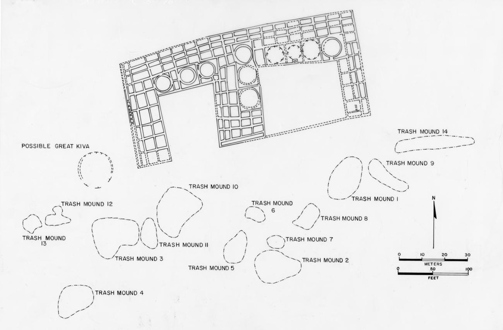Figure 2.8. Kin Bineola Chacoan structure (29SJ 1580; LA 18705) plan view.

Figure 2.9. Kin Bineola Chacoan structure looking west.

¶ 39   The second Chacoan structure component in the Kin Bineola area (29Mc 291; Figures 2.10 and 2.11a, b, c) is at the southern end of the study area overlooking an eastern tributary of Kim-mi-ni-oli Wash. This area was a locus of intensive occupation beginning in ca. A.D. 700 to 880 (DG 200) and continuing through A.D. 1130 (DG 400). The Chacoan structure is quite small—26 by 22 meters, 9 visible and 13 estimated rooms—but the mound height (1.75 meters), the presence of compound and core/veneer masonry, and the relatively large size of some of the visible rooms combine to suggest that this is, in fact, a Chacoan structure. Two probable kiva depressions were noted to the south of the structure, and one room in the roomblock is described as being a possible blocked-in kiva as well. Three good-sized trashmounds (the largest 19 by 18 meters and 1 meter high) and one surface trash concentration were also noted on the site.

Figure 2.10. 29Mc 291 Chacoan structure plan view.

Figure 2.11a. 29Mc 291, Roomblock 1, looking northeast.

Figure 2.11b. 29Mc 291, view of western portion of Roomblock 1 looking northwest.

Figure 2.11c. 29Mc 291, close-up of exposed masonry in southwest corner of Roomblock 1.

¶ 40   This site lies just south of a small tributary wash separating it from 29Mc 261, the village site with an associated great kiva. The great kiva component at 29Mc 261 dates between A.D. 750-1000 and was placed in the 700 to 1025 date group (DG 250), while the Chacoan structure component at 29Mc 291 is dated between A.D 925-1100 and was placed in the A.D. 890 to 1025 (DG 300) and 1030 to 1130 date groups (DG 400). Thus, there is some temporal overlap, but in general 29Mc 291 is the later site. Two of the trash deposits at 29Mc 291 are in the A.D. 890 to 1025 date group, but the refuse associated with the Chacoan structure and the rest of the trash deposits are in the A.D. 1030 to 1130 (DG 400) date group.

¶ 41   The only Chacoan structure (29SJ 2384) recorded in the Chacra Mesa study area is the badly eroded foundation of a great house containing perhaps 40 rooms on the west bank of the Chaco Wash just below Shabik’eshchee Village (see Figures 9.2 and 9.3; also Mathien 2005: Figure 1.5). The isolated great kiva component (site 29SJ 2557) lies higher up in the same rincon. This site was investigated in 1926 or 1927 by Frank H. H. Roberts, Jr., but very little information is available concerning these excavations. Roberts (1929) suggested that the foundations that remain at this site represent a structure that was begun but never completed. An earlier site lies under the great house ruin; the remains of this earlier occupation can be seen eroding from the arroyo bank beneath the south end of the later pueblo. Except for five concentrations of rock, no other features were observed at this site. Ceramics analyzed during the survey date from A.D. 800 to 1150, reflecting the multiple occupations of this location.

Artifact Assemblages by Component Types

¶ 42   Tables 2.7 and 2.8 summarize the artifact assemblages recorded for the different component types. (Note that component types represented by a single example—road associated structures and the fieldhouse/water control type—have been omitted along with rock art sites, and the “other” and “unknown” categories.) These data differ from the summaries presented in the artifact-specific tabulations (ceramics, Chapter 4, and lithics, Chapter 5) in that the feature was the unit of analysis for those studies. Most of the summaries presented in the ceramic and lithic chapters are by feature type; where summaries at the level of a larger spatial unit are presented, they concern whole sites—many of which have more than one temporal or functional component. The data presented here are summarized at the level of these temporal/functional components.

Table 2.7. Ceramic assemblages recorded for the various component types.

Table 2.8. Lithic assemblages recorded for the various component types.

Ceramics

¶ 43   Tables 2.9 and 2.10 show the relative positions of the various component types in terms of selected attributes of the ceramic assemblages. These tables use the summarized assemblage data for all components of a specific type to assess differences and similarities among component types assigned; a subsequent section of this chapter will evaluate the site typology used for the survey using a computerized cluster analysis and other techniques.

Table 2.9. Component types ranked by proportions of vessel forms and ware categories.

Table 2.10. Component types ranked by proportions of nonlocal ceramics.

¶ 44   In interpreting Tables 2.9 and 2.10 it is important to keep in mind the information about numbers of components and numbers of ceramics provided in Table 2.7. In cases where extreme proportions are recorded for component types of which only a small number of examples were included in the analysis (road/trail, cist/storage, Chacoan structure, and great kiva components), or for types that yielded relatively few sherds (shrine, great kiva, water control, cist/storage, and hearth components), these extreme values are as likely to be a function of the small sample as they are to be a result of actual characteristics of components of that type.

¶ 45   With these cautions in mind, a few observations can be offered about the nature of the ceramic assemblages associated with the various component types and about the similarities and differences among some of those types. It is clear from Table 2.9 that there are certain types of components—ceramic scatter, baking pit, hearth, cist/storage, and shrine—whose ceramic assemblages are dominated by jar forms, both in general and in the decorated wares. That this jar dominance is a result of a combination of plainwares (plain gray and corrugated jars) and decorated (painted) wares is evident from the information in the third column of Table 2.9, which shows that, of the five types with the highest jar proportions, only the baking pit component type is among the five types with the highest proportion of plainwares. The four component types with the highest proportions of plainware ceramics in their assemblages (habitations, Chacoan structures, and the two artifact scatter with features categories) have relatively high proportions of bowls in their decorated assemblages so that their overall jar proportion is only moderate. If we examine the component type assemblages with regard to these two variables—proportion of plain to decorated ceramics and proportion of bowls and jars in the decorated assemblages—we find that a majority of the types fall into one of the four logical extremes as follows:

high plain/high bowls	low plain/high bowls
habitation	great kiva
scatter with slabs	water control
scatter with hearth
high plain/low bowls	low plain/low bowls
baking pit	ceramic scatter
hearth	shrine

¶ 46   The major component types that do not fit into these extremes are Chacoan structures, which have a high proportion of plainwares like habitations but a lower proportion of bowls; fieldhouses, which have a moderate proportion of plainwares but a bowl proportion similar to that of habitations; ceramic and lithic scatters, which also have a moderate proportion of plainware but have a markedly lower proportion of bowls than the fieldhouse components; and ledgerooms, which have a relatively low proportion of plainwares but a moderate bowl proportion.

¶ 47   The strongest resemblances among component types in terms of vessel ware/form proportions are those between baking pit and hearth components and between the two artifact scatter with features types. The former are so similar ceramically that it would appear that similar activities were being carried out on sites of these types, or at least that those activities that involved use of ceramics were similar.

¶ 48   Table 2.7 and 2.10 show that trachyte-tempered ceramics and nonlocal ceramics of other sorts appear in quite different proportions on components of some types. Chacoan structures, for example, have the highest relative proportion of trachyte ceramics but a rather low proportion of other imports; shrine components exhibit a similar pattern. The two great kiva components, on the other hand, have very high proportions of other imports but only moderate proportions of trachyte-tempered wares. Water control and cist/storage components have high proportions of other imports and very low proportions of trachyte wares, but again the numbers of components and the numbers of sherds are quite low. Hearths and baking pit components are very low in both types of imports, while fieldhouse and ceramic and lithic scatter components are high in both import categories.

Lithics

¶ 49   Table 2.8 shows that the summarized lithic assemblages recorded for all the components of each type are generally similar to each other. As discussed in the lithic analysis (Chapter 5), Cameron and Young found a good deal of uniformity in the lithic assemblages, but by combining all site types into larger categories—habitations, Chacoan structures, great kivas, small structures, and nonstructural sites—they were able to identify some potentially meaningful variability. Because one of the main purposes of our research was to assess the site typology, we have not used these combined categories, and therefore our conclusions will vary somewhat from theirs.

¶ 50   Cameron and Young also successfully identified some variability among the six grouped site types in the proportions of different classes of debitage (angular debris, primary flakes, secondary flakes, and biface thinning flakes). Because of a change in recording procedures part way through the survey, there is some difficulty in comparing the Kin Klizhin assemblages with those from other survey areas in regard to classes of debitage. For this reason we chose to use “debitage” as a single category of lithic remains for the settlement pattern and site typology portion of the research. The reader is referred to the lithics chapter (Chapter 5) for a more detailed analysis of the variability in proportions of debitage classes among the grouped site types.

¶ 51    It is our impression that much of the assemblage diversity indicated in Table 2.8 is a result of differences in assemblage size. All cases of unusually large or small proportions of a particular lithic class in Table 2.8 occur in component types with small sample sizes. Lithic material type information was also summarized by component type, and the same relationship between assemblage size and diversity was observed. The larger the assemblage, the greater the number of kinds of lithic materials included in that assemblage, regardless of component type.

¶ 52   The lithic ratios shown in Table 2.11 indicate a similar relationship between diversity and assemblage size—nearly all of the extreme values in this table occur in the smaller assemblage categories. There are techniques for assessing differences of diversity among assemblages of different sizes (e.g., Kintigh 1984), but such an analysis was beyond the scope of this chapter. The reader is again referred to the lithics chapter.

Table 2.11. Lithic ratios by component type.

¶ 53    A few of the ratio scores shown in Table 2.11 may well be a result of functional differences among the component types. The relatively extreme values for Chacoan structure components, for example, are likely to be a result of functional differences between these components and those of other types, as Cameron and Young suggest, but they could also be a reflection of the small number of Chacoan structure components included in the sample. The extreme scores for the scatter with hearth components for both debitage/cores and chipped stone tools/groundstone tools may be significant. Because this component type has one of the larger assemblage sizes, extreme values are less likely to be a result of sampling problems. Given that baking pit and hearth components and scatter with slabs and scatter with hearth components form very similar pairs relative to the ceramic data, the differences in lithic assemblages between the members of these pairs may also be significant.

Spatial Variability

Component and Feature Data

¶ 54   Once the overall characteristics of the various component types had been determined, the spatial and temporal variability in these characteristics were examined. Table 2.5 presented information on the numbers and proportions of components of each type within each survey area; Table 2.12 presents similar information about the percentage of the components of each type within each survey area. These two tables make it clear that the prehistoric land-use patterns, at least in the Kin Klizhin, Kin Bineola, and Chacra Mesa survey areas, were quite different. The small size of the South Addition survey area and the concomitantly small number of sites recorded for that area make any interpretation concerning the patterns of use in that area highly tenuous; in general it appears that the area now called the South Addition was used in ways most similar to those apparent for the Kin Klizhin survey area.

Table 2.12. Distribution of each Anasazi component type across the survey areas.

¶ 55   The total number of hectares surveyed was 2,517 (6,220 acres): 20.6 percent of this land was in the Kin Klizhin area (518 ha [1,280 acres]), 17.7 percent in Kin Bineola (445 ha [1,100 acres]), 53.4 percent on Chacra Mesa (1,346 ha [3,325 acres]), and 8.3 percent in South Addition (208 ha [515 acres]). In terms of the proportion of all Anasazi components recorded, therefore, Kin Klizhin has slightly fewer than would be expected based on its size; Kin Bineola has slightly more; and the other two areas have approximately what would be expected. In terms of individual component types, however, Table 2.12 shows many cases in which the percentages of specific component types are markedly out of proportion to the size of the survey area and to the total number of Anasazi components in that area.

¶ 56   Chacra Mesa, for example, contains slightly over 50 percent of all components, but only 27.8 percent of the habitations and 25.0 percent of the fieldhouses. Scatter with slab components are also poorly represented on Chacra Mesa, but scatter with hearth components are not. Kin Bineola, on the other hand, contains only 21.4 percent of all components but has 37.6 percent of the habitations, 63.9 percent of the ledgeroom components, and three of the five Chacoan structure components (although one of these is actually a trash mound associated with the Kin Bineola great house); Kin Klizhin has only 18.2 percent of all components but has 47.2 percent of the fieldhouses and 40.0 percent of the water control components. Over-represented component types on Chacra Mesa include rock art and trails, which is to be expected given the topographical settings of the four survey areas, and baking pits and hearths, which may also be expectable, given the availability of wood on Chacra Mesa.

¶ 57   Table 2.13 presents mean size data for components of each type by area. It would appear from this table that there is considerable variability among areas in this measure, but it is difficult to say how much reliance should be placed on these figures. For single component sites the component size value was taken from the site size as indicted on the survey form. Any variability in how site boundaries were defined both between crews and between field seasons would affect these figures strongly. For multicomponent sites, component size was measured as accurately as possible from the survey form site map. Any inaccuracy in the maps would have been carried over into the component size measurement, and in any case these measurements were at best approximate.

Table 2.13. Mean component size (m2) data by survey area.
Component Type	Kin Klizhin	Kin Bineola	Chacra Mesa	South Addition
Habitation	3,594.2	3,861.2	27,319.4	3,462.1
Fieldhouse	1,351.2	3,408.3	8,697.1	2,871.3
Ledgeroom	-	4,197.7	1,079.3	594.0
Sherd scatter	18,693.2	426.0	2,770.0	3,394.0
Sherd and lithic scatter	770.6	1,120.0	2,604.4	1,588.4
Hearth	1.0	4.0	5,686.5	1,032.0
Baking pit	122.0	1,920.3	16,039.8	135.0
Water control	1,297.8	4,865.9	1,011.2	2,800.0
Cist/storage	3.8	111.6	510.2	25.0
Shrine	694.5	1,947.3	2,100.8	-
Chacoan structure	12,000.0	18,599.4	1,304.0	-
Scatter with slabs	2,266.3	3,842.0	551.7	1,552.1
Scatter with hearth	4,277.4	4,190.8	9,058.5	1,284.9

¶ 58   Even with these cautions in mind, the far greater mean size for habitation components on Chacra Mesa appears to be significant, as do the greater sizes of the hearth and baking pit components in this survey area. The scatter with slab components appear to be unusually small as well as relatively rare on Chacra Mesa, while the scatter with hearth components are larger in this area as well as relatively more abundant than in the other survey areas. The extremely large mean size for ceramic scatter components in Kin Klizhin is the result of a single very large component, as is the unusually large mean size for water control components in Kin Bineola.

¶ 59   One possible explanation for the relatively larger mean size of habitations on Chacra Mesa is related to the relative proportion of pithouse sites among the habitations. If we again divide the habitation components into those components with only pithouses, those with both pithouses and roomblocks, and those with only roomblocks, the proportions of these subtypes are quite different among the three main survey areas. On Chacra Mesa 48.6 percent of the habitations have only pithouses, 37.8 percent have only roomblocks, and 13.5 percent have both types of residential structures. In Kin Bineola 14.0 percent have pithouses only, 44.0 percent have roomblocks only, and 42.0 percent have both. In Kin Klizhin only 9.7 percent have pithouses only, 54.8 percent have roomblocks only, and 35.5 percent have both.

¶ 60   Other aspects of the habitation components also differ from area to area. Among the roomblock features the range of estimated rooms is lowest in Kin Klizhin (range=1-10) and highest in Kin Bineola (1-25 rooms), with Chacra Mesa having a range of 3-20 and South Addition a range of 2-20. A similar pattern is apparent in the mean feature area data for roomblocks: for Kin Klizhin, mean roomblock area is 83.8 square meters, for Kin Bineola it is 263.7 square meters, for Chacra Mesa it is 232.1 square meters, and for South Addition it is 161.6 square meters.

¶ 61   Trash mounds are most common and largest in Kin Bineola (for 43 roomblock and roomblock/pithouse components, trash mound statistics are n=19 and mean area 810.8 square meters), most rare and smallest on Chacra Mesa (for 29 roomblock and roomblock/pithouse components, trash mound n=5 and mean area=272.0 square meters). Again, the apparent anomaly of Chacra Mesa having the largest mean habitation size but the smallest and least numerous trash mounds appears to be related to the high proportion of pithouse-only components in this area. Trash disposal on pithouse sites seems not to have taken place in such a way that mounds were created.

¶ 62   Except for the larger proportion of fieldhouse components in Kin Klizhin, components of this type appear generally similar from area to area, averaging between 1.3 and 1.5 estimated rooms per structure. The mean size of fieldhouse components in the Chacra Mesa area is larger than those for other areas, however. The meaning of this observation is unclear, especially given the very approximate techniques used to derive the component size data. The relatively low proportion of habitation sites on Chacra Mesa may mean that fieldhouses there were more distant from the home site than they were in other areas and thus were occupied for a longer portion of the agricultural year, creating larger surrounding site scatters.

¶ 63   Ledgeroom components are not only much more numerous in Kin Bineola than in other areas, they are larger there as well, averaging 1.5 estimated rooms per structure as opposed to 1 room in the other areas. The mean size data in Table 2.13 also indicate that the Kin Bineola ledgeroom components tend to be larger than those in other areas.

Artifact Data

¶ 64   Table 2.14 provides data on the proportions of different kinds of ceramics broken down both by component and by survey area. This table makes it clear that among components of a single type, there can be marked variability from area to area. There are certain patterns to this variability, however. All component categories have higher proportions of trachyte-tempered ceramics in Kin Klizhin than they do in the other survey areas. In general, the Chacra Mesa component categories have higher proportions of plainwares (both plain gray and corrugated vessels) than do the same categories in other survey areas. Table 2.14 provides data on the proportions of different kinds of ceramics broken down both by component and by survey area. This table makes it clear that among components of a single type, there can be marked variability from area to area. There are certain patterns to this variability, however. All component categories have higher proportions of trachyte-tempered ceramics in Kin Klizhin than they do in the other survey areas. In general, the Chacra Mesa component categories have higher proportions of plainwares (both plain gray and corrugated vessels) than do the same categories in other survey areas.

Table 2.14. Ceramic assemblages recorded for the various component types by area.

¶ 65   Certain component categories exhibit a greater regularity from area to area than do others. Chacoan structure components, for example, are quite similar to one another, although the number of components involved is very small. The baking pit component assemblages from Kin Bineola and Chacra Mesa (the only areas with components of this type that occur in any numbers) are very similar.

¶ 66   These area to area differences among components of the same type have two possible explanations: either the criteria for assigning components to a type are inadequate in terms of grouping similar phenomena together and separating dissimilar phenomena, or some factor other than component type is differentially affecting the ceramic assemblages from area to area. As will be discussed in the section below on evaluating the site typology, it is our opinion that the latter explanation is correct. We will suggest that temporal factors account for a significant portion of the area to area variability among components of the same type. Temporal factors may account, for example, for the higher proportion of plainwares in the Chacra Mesa components, because that area has the highest proportion of very early sites. Likewise, the higher proportion of trachyte-tempered material in Kin Klizhin may, at least in part, be a reflection of the preponderance of A.D. 1030 to 1130 (DG 400) components in that area.

¶ 67   Lithic data for both material types and morphological categories were also examined relative to survey area. Unlike the ceramic assemblages, the lithic assemblages exhibited little variability between survey areas that could not be attributed to differences in assemblage size. The few identifiable differences tended to be between Kin Bineola and the other three survey areas, a finding expanded upon by Cameron and Young in Chapter 5.

Temporal Variability

¶ 68   There are two ways to look at the temporal data for the archaeological components identified during this survey, both of them based on ceramics. The ceramic analysis (Chapter 4) yielded temporal information both in the form of date groups (Table 2.2)—time spans within which a given ceramic assemblage dates based on the constellation of ceramic types—and beginning and ending dates—the earliest possible and latest possible data for an assemblage, based on individual ceramic types present. Date groups and ceramic beginning dates provide related but complementary perspectives on change through time in the project area. Tables displaying a) numbers of components of each component type by date group and beginning date and b) total numbers of components in each survey area by date group and beginning date are provided in Appendix 2.3.

¶ 69   In order to preserve as much information as possible, all date groups and all component types are included in the tables in Appendix 2.3. From a practical standpoint, however, the large number of categories in these tables makes them difficult to interpret. In an attempt to present these temporal data in a more manageable, if less fine-grained form, Tables 2.15 and 2.16 were created to show numbers of components of each type by major date group and numbers of selected component types by beginning dates. The major date groups [A.D. 550 to 750 (DG 100), A.D. 700 to 880 (DG 200), A.D. 890 to 1025 (DG 300), A.D. 1030 to 1130 (DG 400), and A.D. 1130 to 1230 (DG 500)] account for nearly 90 percent of the components for which date group information is available, so Table 2.15 gives a fairly complete picture of the temporal trends in component types relative to the date groups established during the ceramic analysis. In order to examine the beginning date trends we eliminated “other” and “unknown” components from Table 2.16 along with any other component types with fewer than 12 cases (half the number of beginning date categories).

Table 2.15. Distribution of component types by date group.

¶ 70   Two important factors should be kept in mind when examining Table 2.15 and when reading this entire discussion of temporal variability. The date groups defined during the ceramic analysis are not the same length, and two of them [A.D. 550 to 750 (DG 100) and A.D. 700 to 880 (DG 200)] overlap slightly. The differential lengths of the date groups means that the actual preponderance of components in this sample dating to A.D. 1030 to 1130 (DG 400) is even greater than it appears to be in Table 2.15 and that the sparseness of A.D. 700 to 880 (DG 200) occupation is even more marked than it appears from the table. If the numbers of components per date group shown in the total row at the bottom of Table 2.15 were normalized to numbers of datable components per year of the estimated time span for each date group, the results are as follows: A.D. 550 to 750 (DG 100), 0.4 components per year; A.D. 700 to 880 (DG 200), 0.2 components per year; A.D. 890 to 1025 (DG 300), 0.8 components per year; A.D. 1030 to 1130 (DG 400), 2.0 components per year, and A.D. 1130 to 1230 (DG 500), 0.3 components per year.

Component Type Data

¶ 71   Table 2.15 shows that between A.D. 550 to 750 (DG 100), settlement in the survey areas consisted largely of habitation and scatter with hearth components; more than 20 percent of the identified components of these two types date to this period while only 9.7 percent of all components are assigned to this time. Between A.D. 700 to 880 (DG 200) settlement was still heavily dominated by a disproportionate number of habitation components, and fieldhouse and ledgeroom components are also somewhat over-represented. Overall, the intensity of occupation as measured by the number of components, and as measured by the numbers of components per year, declined markedly during this period.

¶ 72   During the A.D. 890 to 1025 (DG 300) period the pattern of prehistoric land-use in the survey area changed. The intensity of occupation as measured by the number of components increased dramatically, the variety of component types increased, and for the first time the settlement system was dominated not by habitation components but by fieldhouses and a variety of nonstructural sites—especially ceramic and ceramic and lithic scatters and baking pit components, along with the two scatter with features component types.

¶ 73   The most intensive use of the survey area occurred between A.D. 1030 to 1130 (DG 400). As in the A.D. 890 to 1025 (DG 300) period, a variety of component types were in use. Habitations again became the most prevalent component type, but fieldhouses, ledgerooms, ceramic and lithic scatters, and scatter with slab components occur in their greatest numbers and highest proportions during this time.

¶ 74   Between A.D. 1130 and 1230 (DG 500), occupation of the survey area declined drastically. A few habitations and fieldhouses were occupied during some part of this period, but in general use of the area was extremely sparse during this 100-year period.

¶ 75   Some interesting patterns suggestive of possible functional relationships between component types appear in Table 2.15. Habitation sites, for example, occur in the largest numbers between A.D. 1030 and 1130 (DG 400), with their second largest number between A.D. 550 and 750 (DG 100). The only other component category of any size that exhibits this same pattern is the scatter with hearth category (hearth components occur in the same relative proportions, but the numbers involved are very small). This could indicate that the use of the scatter with hearth components was somehow related to the occupations of habitation components or it could be that the scatter with hearth components represent unrecognized habitation sites—possibly pithouse sites given the A.D. 550 to 750 (DG 100) emphasis. Components were assigned to the scatter with hearth category on the basis of the presence of burned slabs or fire-cracked rock, as well as in cases where actual hearths were visible. Pithouses are frequently found to have been burned at or after abandonment, and surface indications in the form of burned elements often occur along with the diagnostic surface depressions.

¶ 76   As another example, nearly half of the fieldhouse components occur in the A.D. 1030 to 1130 (DG 400) period; approximately an additional one-quarter occur in the A.D. 890 to 1025 (DG 300) period. A very similar pattern is apparent for the ceramic and lithic scatters and the scatter with slabs components. Again, this may suggest that these three component types were functionally complementary parts of the settlement system or that at least some of these apparently nonstructural sites functioned as fieldhouses.

¶ 77   The beginning date information in Table 2.16 is based on the earliest ceramic beginning date offered for any feature included within a given component. In one sense this gives a false picture of the temporal pattern of component occupation because whole components are assigned to the date of the earliest single feature. On the other hand, this practice provides at least some temporal placement (in the form of a “no earlier than” statement) for components that could not be assigned to a date group and therefore appear only in the “other” column in Table 2.15.

Table 2.16. Distribution of component types by beginning date.

¶ 78   In general the beginning date information supports the observations made concerning the date group patterns. Habitation components again exhibit an early, mid-sixth century peak and a late, early to mid-eleventh century peak. Scatter with hearth components once more have peaks during the same two periods, but the addition of components that could not be assigned to a single date group has significantly increased the representation of this type in the earliest time period. This would seem to support the suggestion that these scatter with hearth components may be unrecognized pithouse sites, because it is pithouse-only components that create the early peak in habitation component frequencies. The temporal distribution of hearth components again closely resembles that of habitations and scatter with hearth components, but as noted before, the numbers involved are quite small.

¶ 79   Fieldhouses have frequency peaks in the tenth and eleventh centuries as the date group information would suggest. The ceramic and lithic scatter components again resemble the fieldhouses in their temporal distribution, but the addition of several components that could not be assigned to date groups to the early end of the temporal sequence for the scatter with slabs category decreases the resemblance between this component type and fieldhouses somewhat. Scatter with slab components still exhibit a mid-tenth to mid-eleventh century peak, but they also have a small early sixth century peak; it is possible that some of these early scatter with slab components also represent unrecognized pithouse sites.

¶ 80   The date group information indicated that baking pits were the only component type that did not occur in greatest numbers between A.D. 1030 and 1130 (DG 400), and this pattern is even clearer in the beginning date information. Whatever the function of these sites, they were more important before A.D. 1025 than they were during the major (A.D. 1030 to 1130; DG 400) occupation of the survey area.

¶ 81   Table 2.16 indicates that ledgerooms, more than any other component category, were a phenomenon of the eleventh century. The water control components also tend to date to this time, but the small numbers involved and the large proportion of undated components of this type preclude any definite statement to this effect.

¶ 82   Major component categories that do not appear in Table 2.16 include rock art and stairway components because none of these were dated, and the great kiva and Chacoan structure components. As noted in the individual descriptions of these latter components, the Kin Bineola great kiva dates to A.D. 700 to 1025 (DG 250) and the Chacra Mesa one to A.D. 1130 to 1230 (DG 500). The outlier site of Kin Klizhin dates to A.D. 1030 to 1130 ( DG 400), the Kin Bineola outlier and the smaller Chacoan structure that lies near the south end of the Kin Bineola survey area both date to A.D. 890 to 1130 interval (DG 300 and 400), and the never completed Chacoan structure below Shabik'eshchee Village in the Chacra Mesa study area cannot be precisely dated because ceramics from its occupation have mixed with sherds from an underlying site located in the same place. The range of pottery on the site is dated between A.D. 800-1150, suggesting an end date for the Chaco structure of no later than 1150.

Feature Data

¶ 83   Table 2.17 shows the results of breaking down the habitation components into subtypes of pithouse only, roomblock only, and both roomblock and pithouse, by date group. The temporal differentiation between the early pithouse only and late roomblock only subtypes is so marked that it seems likely that at least some of the seven early roomblock only components actually have pitstructures on them that are no longer visible.

Table 2.17. Habitation component subtypes by date group.
	Habitation Component Subtypes
Date Group (A.D.)	Pithouse Only		Roomblock Only		Both Roomblock and Pithouse
	No.	%a	No.	%	No.	%
550-750	19	55.9	1	1.8	8	18.2
700-880	8	23.5	1	1.8	8	8.2
700-1025	1	2.9	1	1.8	7	15.9
890-1025	4	11.8	4	7.3	8	18.2
890-1130	-	-	-	-	2	4.5
1030-1130	-	-	39	70.9	6	13.6
1030-1230	-	-	2	3.6	-	-
1130-1230	-	-	5	9.1	-	-
Otherb	2	5.9	2	3.6	5	11.4
TOTAL	34		55		44
aPercent of all components of this subtype in this data group. bIncludes both date group unknown and multiperiod hybrid date groups.

¶ 84   Table 2.18 shows the temporal patterning in visible and estimated room data for roomblocks, fieldhouses, and ledgerooms. This table shows that roomblock features experienced a slight decrease in size during A.D. 700 to 880 (DG 200) just as habitation components, and indeed components of all types, experienced a decrease in numbers. In general, however, both roomblocks and ledgerooms show a pattern of increasing size over time until A.D. 1030 to 1130 (DG 400), after which the size of these structures as well as the number of components decreases. Fieldhouses, on the other hand, remain quite constant over time in the matter of numbers of rooms.

Table 2.18. Mean visible and estimated room counts by date group.
	Mean Visible and Estimated Room Counts
Date Group (A.D.)	Roomblock		Fieldhouse		Ledgeroom
	Visible	Estimated	Visible	Estimated	Visible	Estimated
550-750	3.1	4.7	1.5	1.3	-	-
700-880	2.5	4.1	1.0	1.2	1.0	1.0
890-1025	2.2	8.1	1.1	1.4	1.2	1.2
1030-1130	3.3	8.0	1.1	1.5	1.5	1.7
1130-1230	4.0	6.2	1.5	1.6	1.0	1.1

¶ 85   Mean feature area data (Table 2.19) for roomblocks exhibit the same pattern of a slight decrease in A.D. 700 to 880 (DG 200) followed by increases in A.D. 890 to 1025 (DG 300) and A.D. 1030 to 1130 (DG 400) followed by another decrease in A.D. 1130 to 1230 (DG 500). Ledgerooms also show a pattern similar to that indicated by the visible and estimated room data, but fieldhouses do not. Although the numbers of rooms indicated for fieldhouse features do not vary markedly with time, the size of these features does. The survey data indicate that fieldhouses reached their greatest size during A.D. 890 to 1025 (DG 300), the period during which their numerical importance in the settlement system equaled that of habitation components.

Table 2.19. Mean feature area data by date group.
Date Group (A.D.)	Mean Feature Area in Square Meters
	Roomblock	Fieldhouse	Ledgeroom
550-750	98.8	9.7	-
700-880	70.7	9.2	8.4
890-1025	164.4	44.2	7.0
1030-1130	256.2	25.8	17.3
1130-1230	193.3	11.0	11.3

Differences Among Survey Areas

¶ 86   Table 2.20 presents data on the distribution of components assigned to the major date groups by survey area. It is clear from this table that Chacra Mesa has a disproportionate share of the A.D. 550 to 750 (DG 100) occupation and of components that could not be dated or could not be assigned to a single date group, along with a low proportional representation for A.D. 700 to 880 (DG 200). That is, approximately 5 percent of components from all areas date to the A.D. 700 to 880 (DG 200) period, but on Chacra Mesa only 2 percent of all components date to this time. The South Addition also appears to be high in A.D. 550 to 750 (DG 100) and low in A.D. 700 to 880 (DG 200) as well as being very high in A.D. 890 to 1025 (DG 300). This area contained no sites dated to A.D. 1130 to 1230 (DG 500). Kin Klizhin and Kin Bineola, on the other hand, have a very low proportion of A.D. 550 to 750 (DG 100) components , and Kin Bineola has a very high proportion of A.D. 700 to 880 (DG 200) components. Kin Klizhin, by contrast, is high in A.D. 1030 to 1130 (DG 400) and A.D. 1130 to 1230 (DG 500) components.

Table 2.20. Number of components in major date groups by survey area.
Date Group (A.D.)	Kin Klizhin		Kin Bineola		Chacra Mesa		South Addition		Total
	No.	%a	No.	%	No.	%	No.	%
550-750	5	7.0 (3.8)	8	11.3 (5.1)	48	67.6 (12.7)	10	14.1 (15.9)	71 (9.7)
700-880	8	22.2 (6.0)	19	52.8 (12.2)	8	22.2 (2.1)	1	2.8 (1.6)	36 (4.9)
890-1025	22	19.6 (16.5)	23	20.5 (14.7)	47	42.0 (12.4)	20	17.9 (31.8)	112 (15.3)
1030-1130	60	30.5 (45.1)	49	24.9 (31.4)	74	37.6 (19.6)	14	7.1 (22.2)	197 (27.0)
1130-1230	10	38.5 (7.5)	2	7.7 (1.3)	14	53.9 (3.7)	0	- -	26 (3.6)
Otherb	28	9.7 (21.1)	55	19.1 (35.3)	187	64.9 (49.5)	18	6.3 (28.6)	288 (39.5)
TOTAL	133	18.2	156	21.4	378	51.8	63	8.6	730
aPercentage of all components of this date group (row) and, in parentheses, the percentage of all components in this area that are this date group (column). bIncludes both hybrid date groups and no date group components.

¶ 87   Because A.D. 550 to 750 (DG 100) components tend to be dominated by habitations (Table 2.15), the heavy representation of A.D. 550 to 750 ( DG 100) components on Chacra Mesa and in the South Addition means that an unusually large proportion of all habitation components in those areas date to A.D. 550 to 750 (DG 100). A computer search of the data base revealed that on Chacra Mesa 48.4 percent of all habitation components are A.D. 550 to 750 (DG 100); in South Addition 41.7 percent of the habitations date to this period. In Kin Klizhin and Kin Bineola, by contrast, only 7.3 and 14.3 percent of the habitations, respectively, are between A.D. 550 and 750 (DG 100). Interestingly, this same computer search indicated that the scatter with hearth components exhibit the same pattern, being disproportionately represented in A.D. 550 to 750 (DG 100) on Chacra Mesa and in the South Addition, but not in Kin Klizhin and Kin Bineola. We also found that fieldhouse and scatter with slabs components tend to be heavily over-represented in A.D. 1030 to 1130 (DG 400) in Kin Klizhin and Kin Bineola but not on Chacra Mesa or in South Addition. Most other component types are represented in roughly the same proportions from date group to date group for all areas.

¶ 88   In the computer search we also inspected the proportion of the various subtypes for habitations. As would be expected from the higher proportion of A.D. 550 to 750 (DG 100) components, Chacra Mesa and South Addition have much higher proportions of pithouse-only components among their habitation sites. Chacra Mesa has 48.6 percent pithouse-only components and 37.8 percent room-block components, with 13.5 percent of the habitation components having both types of residential structures. South Addition has 40.0 percent pithouse only, 13.3 percent roomblock only, and 46.7 percent both. Kin Klizhin and Kin Bineola have only 9.7 and 14.0 percent pithouse-only components, respectively, with 54.8 and 44.0 percent roomblock-only and 35.5 and 42.0 both pithouse and roomblock components.

Artifact Data

¶ 89   Given that the date group and beginning date assignments for components are based on ceramics, temporal patterning in the ceramic assemblages from components of various types is clearly not an independent phenomenon. Nevertheless, some of the information presented in Table 2.21 is very important for our understanding of ceramic similarity and variability among components of different types. For example, Table 2.21 shows a general pattern of decline in the percentage of plainwares over time; this is especially clear in the habitation, fieldhouse, and scatter with features component types. This means that components of a particular type or in a particular area whose assemblages are heavily dominated by plainwares may be simply earlier than, rather than functionally distinct from, components whose assemblages contain higher proportions of decorated ceramics. Likewise, this table shows ceramic assemblages with higher proportions of imported wares may be later than comparable assemblages rather than being a reflection of differential access to tradewares.

Table 2.21. Ceramic assemblages recorded for the various component types by date group.

¶ 90   Two other interesting trends are apparent in the data displayed in Table 2.21. One is that the temporal distribution of trachyte-tempered ceramics and of other imports is distinctly different. The trachyte wares generally increase over time and peak in A.D. 1030 to 1130 (DG 400) with a fall off in A.D. 1130 to 1230 (DG 500). The other imports, on the other hand, occur in very low proportions in A.D. 550 to 750 (DG 100) through A.D. 1030 to 1130 (DG 400) and exhibit a marked increase in A.D. 1130 to 1230 (DG 500) across all component types. This is apparently a reflection of the influx of Mesa Verdean ceramics late in the Chacoan sequence, but it is interesting to find that this shift in ceramic assemblages occurs across all component types. The second observation that can be made from Table 2.21 is that the patterns for habitation, fieldhouse, and scatter with feature components are quite similar, and that these component types are noticeably different from the other component types. The lithic morphological and material type data were also summarized by date group. The material type information indicated that there was a slightly higher percentage of obsidian in A.D. 550 to 750 (DG 100) assemblages than in assemblages from later time periods and that Washington Pass chert occurred in the highest proportion in A.D. 1030 to 1130 (DG 400) assemblages. The morphological data indicated that the proportion of angular debris in the debitage assemblage increased over time while the proportion of biface thinning flakes decreased. Projectile points and utilized flakes are most common in early assemblages, while hammerstones are most common in later ones. The debitage-to-tool and debitage-to-core ratios shown in Table 2.22 exhibit similar patterns: a slight drop in A.D. 700 to 880 (DG 200) relative to the A.D. 550 to 750 (DG 100) figures, an increase to maximum values in A.D. 890 to 1025 (DG 300), and a decline through A.D. 1030 to 1130 (DG 400) and A.D. 1130 to 1230 (DG 500) to values that are still somewhat above A.D. 550 to 750 (DG 100) levels. The ratio of chipped stone tools to ground stone tools, on the other hand, shows a sharp drop between A.D. 550 to 750 (DG 100) and A.D. 700 to 880 (DG 200) with relatively stable values throughout the subsequent periods.

Table 2.22. Lithic ratios by date group.
Date Group (A.D.)	Debitage/tools	Debitage/cores	Chipped/ground tools
550-750	8.7:1	42.5:1	4.1:1
700-880	7.5:1	31.6:1	1.9:1
890-1025	18.0:1	85.3:1	1.5:1
1030-1130	17.1:1	64.6:1	1.6:1
1130-1230	13.1:1	49.7:1	1.8:1

Geographic Distribution of Components

Kin Klizhin

¶ 91   Figures 2.12 through 2.16 show the distribution of ten major component types (habitation, Chacoan structure/great kiva, fieldhouse, ledgeroom, water control, cist/storage, baking pit, hearth, artifact scatter, artifact scatter with features) over the five major time periods in the Kin Klizhin survey area. In order to preserve as much information as possible, components occupied during two date groups appear on both maps [e.g., components dated A.D. 890 to 1130 (DG 350) appear on both the A.D. 890 to 1025 (DG 300) and A.D. 1030 to 1130 (DG 400 ) maps]. Components spanning more than two date groups and Anasazi components for which no date could be determined do not appear on any of the time period maps.

Figure 2.12. Kin Klizhin survey area: A.D. 550-750 (DG 100) and A.D. 550-880 (DG 150) sites. Total components = 6.

Figure 2.13. Kin Klizhin survey area: A.D. 700-880 (DG 200), A.D. 700-1025 (DG 250), and A.D. 550-880 (DG 150) sites. Total components = 12.

Figure 2.14. Kin Klizhin survey area: A.D. 890-1025 (DG 300), A.D. 890-1130 (DG 350), and A.D. 700-1025 (DG 250) sites. Total components = 25.

Figure 2.15. Kin Klizhin survey area: A.D. 1030-1130 (DG 400), A.D. 1030-1230 (DG 450), and A.D. 890-1130 (DG 350) sites. Total components = 64.

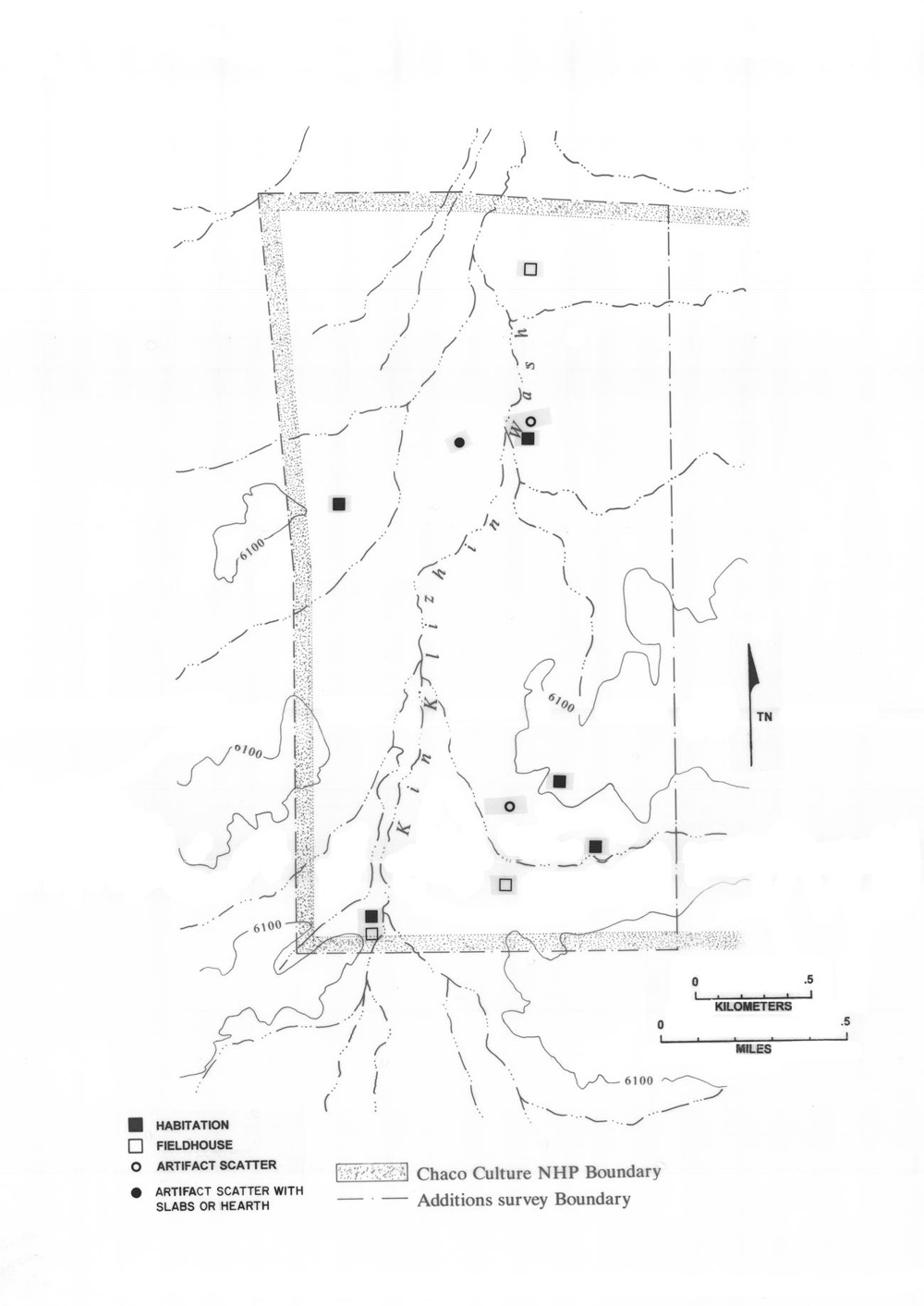Figure 2.16. Kin Klizhin survey area: A.D. 1130-1230 (DG 500) and A.D. 1030-1230 (DG 450) sites. Total components = 11.

¶ 92   Figures 2.17 through 2.19 illustrate the distribution within the Kin Klizhin area of all recorded components of the following functional types: water control components, baking pits and hearths, and shrines, rock art, and road/trail segments and their associated features, such as stairs. Unlike the time period maps (Figures 2.12 through 2.16), these figures show all components of these types recorded in Kin Klizhin. Because so many of these components are undated and/or have no associated artifacts, both components believed to be Anasazi and those assigned to the “unknown” cultural category are included.

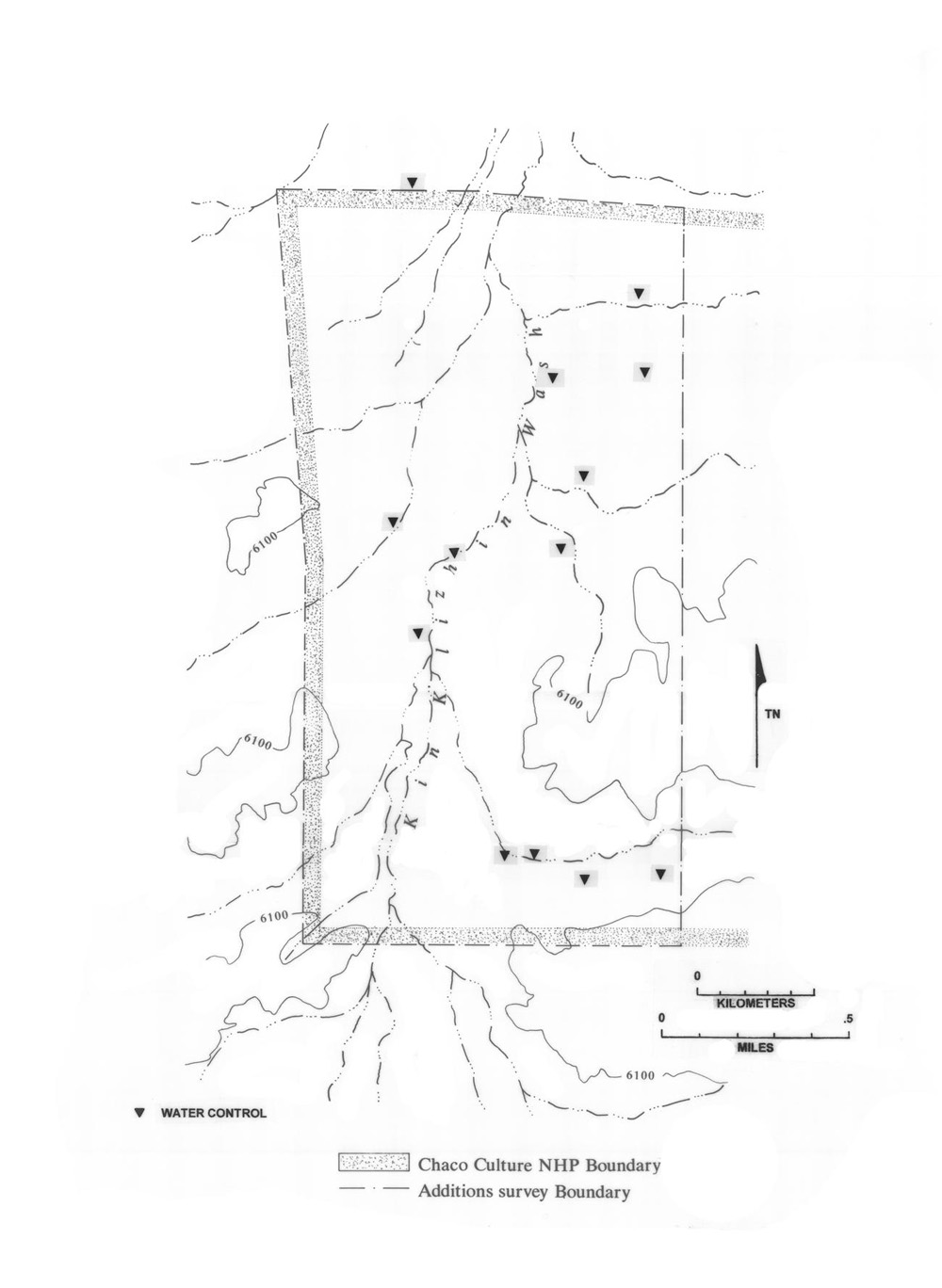Figure 2.17. All Kin Klizhin Anasazi water control components dated and undated. Total components = 13.

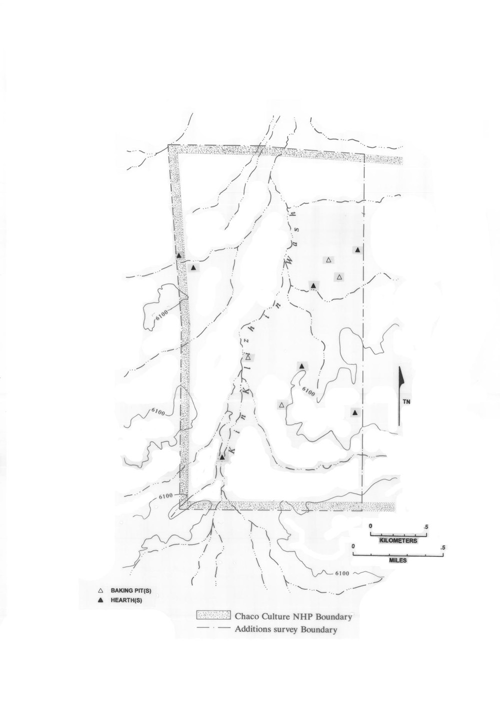Figure 2.18. All Kin Klizhin baking pit and hearth components of Anasazi, Archaic, and Unknown affiliation. Total components = 11.

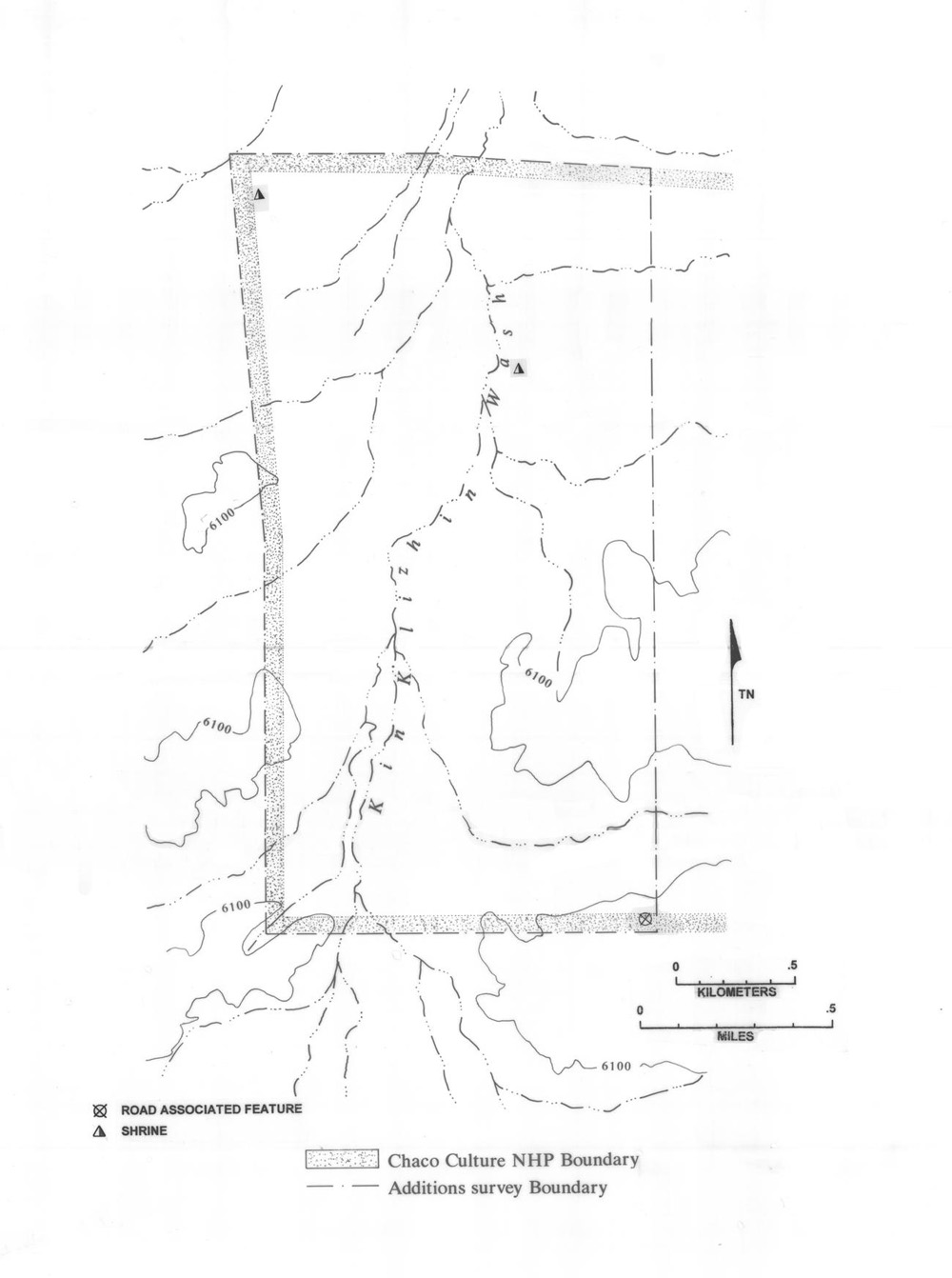Figure 2.19. All Kin Klizhin Anasazi shrine and herradura (road associated) components. Total components = 3.

¶ 93   Figures 2.12 and 2.13 graphically demonstrate the sparseness of occupation in Kin Klizhin during the early period from A.D. 550 to 880. Two habitation components near the north end of the area and three artifact scatter components in the central portion of the area constitute the entire A.D. 550 to 750 (DG 100) occupation. By A.D. 700 to 880 (DG 200), however, three small clusters of habitation components, two in the general area of the A.D. 550 to 750 (DG 100) settlements and a new one near the southern end of the survey area are evident. In addition the area along the eastern slopes of Kin Klizhin Wash was being used nonresidentially by means of fieldhouses.

¶ 94   Figure 2.14 shows that in A.D. 890 to 1025 (DG 300), residential use of the northern, downstream portion of this survey area had been discontinued. The habitation cluster in the central portion of the area was still occupied, however, and residential use of the southern portion of the survey area had expanded. Datable water control components also appear for the first time during this period.

¶ 95   During the A.D. 1030 to 1130 (DG 400) period (Figure 2.15), occupation intensity increased markedly. Some renewed residential use of the northern portion of the survey area is indicated. Habitation components appear along the small eastern tributaries of the wash in the north half of the survey area for the first time, and nonresidential use in the form of fieldhouses increased in both the north and the wash areas. The long-term habitation in the central portion of the survey area culminated in the construction of the Kin Klizhin outlier during this period. The residential use of the extreme southern portion of the area was largely replaced by nonresidential, fieldhouse use, while a series of habitation components appear for the first time in the south-central portion of the survey area—between the earlier central and southern clusters.

¶ 96   With the advent of A.D. 1130 to 1230 (DG 500) (Figure 2.16) the northern portion of the survey area was largely depopulated; a single habitation component, a fieldhouse, and two scatters occur on the floodplain and the eastern slope of the wash. The central portion of the area surrounding the uninhabited Kin Klizhin outlier was also nearly unoccupied. The single exception is a small habitation half a kilometer north of the outlier that has some A.D. 1130 to 1230 (DG 500) ceramics on its trashmound. A small number of habitation and fieldhouse components in the general area of the A.D. 700 to 880 (DG 200) southern cluster constituted most of the A.D. 1130 to 1230 (DG 500) occupation of this survey area.

¶ 97   The water control component map (Figure 2.17) shows that most of these features lie in side drainages entering Kin Klizhin Wash from the east—especially in the area of the southern cluster of habitation components and in the northeastern portion of the survey area—although a large diversion dam and a canal segment and a few other water control features are to be found in the main channel near the Kin Klizhin outlier. It is likely that other water control components once existed in the main channel but have since been washed away.

¶ 98   The baking pit and hearth components22 [CLOSE]The hearths include 2 Archaic, 4 Unknown and 1 Anasazi component. Baking pits include 1 Archaic, 1 Unknown and 2 Anasazi components. (Figure 2.18) appear to be located largely on slopes and higher ground away from the main wash. There were no reported rock art components in Kin Klizhin, perhaps owing to the dearth of suitable locations. There are two shrines (Figure 2.19): one is near the two A.D. 550 to 750 (DG 100) habitation components; the other is in the area of sloping land to the east of Kin Klizhin Wash in the north half of the survey area. No road or trail segments were identified in this survey area, but one component identified as a possible road-associated structure (an herradura) was recorded in the very southeastern corner of the survey unit (Figure 2.19).

Kin Bineola

¶ 99   Figures 2.20 through 2.24 provide information on the distribution of the ten major component types for the five major date groups as was done for Kin Klizhin. Again, components spanning two date groups are included on the maps for both time periods. Figures 2.25 through 2.27 provide information on the distribution of water control, baking pit, hearth, shrine, rock art, and road/trail components. Again, all components of these types are shown, regardless of temporal or cultural affiliation.

¶ 100   Figure 2.20 shows that during the A.D. 550 to 750 (DG 100) period, settlement in the Kin Bineola area consisted of a series of habitation and scatter with feature components (which as noted above may represent pithouse sites) on mesa tops and valley slopes along both sides of Kim-mi-ni-oli Wash, especially in its middle reaches (relative to the boundaries of the survey area). By A.D. 700 to 880 (DG 200) (Figure 2.21) this scatter had resolved itself into three relatively distinct clusters, composed largely of habitation components—one in the north, one in the central reaches mentioned before, and one especially tightly clustered group in the south that included a great kiva component.

Figure 2.20. Kin Bineola survey area: A.D. 550-750 (DG 100) and A.D. 550-880 (DG 150) sites. Total components = 11.

Figure 2.21. Kin Bineola survey area: A.D. 700-880 (DG 200), A.D. 700-1025 (DG 250), and A.D. 550-880 (DG 150) sites. Total components = 27.

¶ 101   The A.D. 890 to 1025 (DG 300) map (Figure 2.22) shows that by this time the settlement pattern in Kin Bineola had further coalesced into two main clusters, one in the north in the vicinity of the Kin Bineola outlier and the other in the south where the A.D. 700 to 880 (DG 200) community was located. A small Chacoan structure and an isolated great kiva formed part of this community, although the great kiva probably dates to the early part of the period while the Chacoan structure dates to the later part. The central part of the survey area was used less intensively during this period, but at least two habitation components and a small number of other structural and nonstructural components are present.

Figure 2.22. Kin Bineola survey area: A.D. 890-1025 (DG 300), A.D. 890-1130 (DG 350), and A.D. 700-1025 (DG 250) site. Total components = 29.

¶ 102   Between A.D. 1030 and 1130 (DG 400) (Figure 2.23), a series of habitation components were occupied along the central and northern portions of the wash above and below the Kin Bineola outlier. A second series of habitations lies along the south-central and southern portions of the wash, with the heaviest concentration at the very southern edge of the survey area. The location of the original, long-occupied southern cluster of habitations surrounding the great kiva is uninhabited by this period, and occupation is centered along the main wash to the south of this original center of occupation.

Figure 2.23. Kin Bineola survey area: A.D. 1030-1130 (DG 400), A.D. 890-1130 (DG 350), and A.D. 1030-1230 (DG 450) sites. Total components = 51.

¶ 103   Figure 2.24 makes the extreme nature of the abandonment of the Kin Bineola area between A.D. 1130 and 1230 (DG 500) very clear. A single habitation and a fieldhouse in the vicinity of the abandoned outlier of Kin Bineola along with a single ledgeroom component in the lone-occupied but not abandoned southern cluster constitute the entire A.D. 1130 to 1230 (DG 500) occupation of the Kim-mi-ni-oli Valley within the survey area.

Figure 2.24. Kin Bineola survey area: A.D. 1130-1230 (DG 500) and A.D. 1030-1230 (DG 450) sites. Total components = 3.

¶ 104   Preserved water control components33 [CLOSE]These include 8 Anasazi and 1 Unknown component. in the Kin Bineola survey area (Figure 2.25) are relatively few in number and generally are located within the main wash itself, a pattern somewhat different from that noted for Kin Klizhin. These water control features include a masonry dam complex across the wash at 29Mc 214 and what appears to be a canal (site 29Mc 341) more than a kilometer long, running from this dam complex to the alluvial flats southwest of the site of Kin Bineola. This canal ends in the vicinity of a massive coursed masonry wall (29Mc 147) of unknown function. The dam and canal are at the heart of a cluster of water control features extending to the north and south. These are discussed extensively in Chapter 9.

Figure 2.25. All Kin Bineola water control components of Anasazi and Unknown cultural affiliation. Total components = 9.

¶ 105   Baking pit and hearth components44 [CLOSE]The hearths include 1 Anasazi and 6 Unknown components. Baking pits include 10 Anasazi and 10 Unknown components. (Figure 2.26) are distributed along the south-central and southern portions of the wash. Their distribution resembles that of other component types in this southern half of the survey area, but the near absence of components of this type in the northern portions of the area is an abrupt departure from the distribution of other component types.

Figure 2.26. All Kin Bineola baking pit and hearth components of Anasazi and Unknown cultural affiliation. Total components = 27.

¶ 106   Shrine and rock art components55 [CLOSE]These include 4 Anasazi shrines, 7 Anasazi rock art components and 1 Unknown rock art component. (Figure 2.27) are clustered in the central reaches of the wash and in the vicinity of the southern habitation cluster. Although the location of the rock art panels is at least partially contingent on the location of suitable rock faces, the close spatial association between rock art and shrines is noticeable and of interest (cf. the map showing this same distribution for Chacra Mesa below).

¶ 107   Road and trail segments and associated component types (Figure 2.27) are virtually absent from the Kin Bineola survey area. The single exception is a possible road segment near the site of Kin Bineola.

Figure 2.27. All Kin Bineola shrine, rock art, and road segment components of Anasazi and Unknown cultural affiliation. Total components =13.

Chacra Mesa

¶ 108   Figures 2.28 through 2.32 illustrate component type distributions for the five major date groups on Chacra Mesa; as in the previous section, components spanning two date groups are shown on both maps. Figures 2.33 through 2.35 show the distribution of water control, baking pit, hearth, shrine, rock art, road/trail and associated components. Components of all time periods and of both Anasazi and “unknown” cultural affiliation appear on these maps.

¶ 109   The A.D. 550 to 750 (DG 100) map (Figure 2.28) shows that most of the residential occupation of Chacra Mesa during this period was concentrated along a single drainage cutting into the north face of the mesa and draining into Chaco Wash. The large and well-known pithouse village of Shabik’eshchee (29SJ 1659; Roberts 1929) lies on a point on the mesa’s north edge, overlooking this drainage and Chaco Wash. Additional habitation components were found on the mesa top near the eastern end of the survey area and along the southern edge of the mesa, also near the eastern end of the survey area. The rest of the survey area appears to have been used sparsely and nonresidentially during this period.

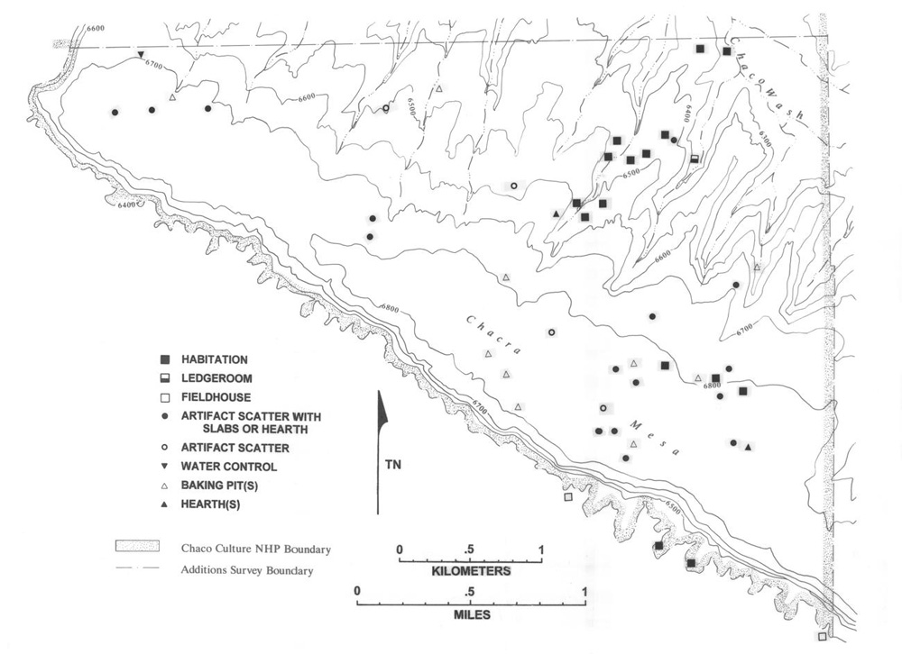Figure 2.28. Chacra Mesa survey area: A.D. 550-750 (DG 100) and A.D. 550-880 (DG 150) sites. Total components = 51.

¶ 110   Between A.D. 700 and 880 (DG 200) (Figure 2.29), occupation of the Chacra Mesa survey area declined sharply. A single habitation on the canyon floor east of Shabik’eshchee Village is the only residential component; a scattering of nonresidential and largely nonstructural components on the northern and southern edges of the survey area constitute the remainder of the occupation.

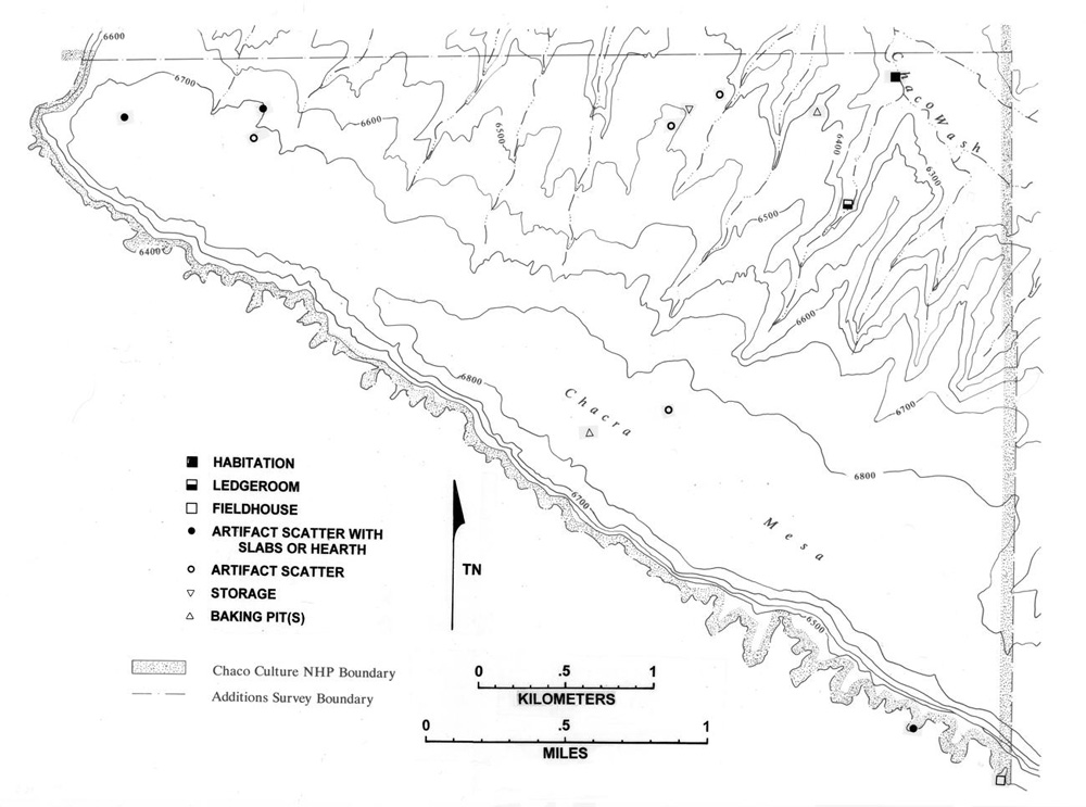Figure 2.29. Chacra Mesa survey area: A.D. 700-880 (DG 200), A.D. 550-880 (DG 150), and A.D. 700-1025 (DG 250) sites. Total components = 13.

¶ 111   Between A.D. 890 and 1025 (DG 300) (Figure 2.30), nonresidential use of the Chacra Mesa survey area increased, largely in the form of baking pit and artifact scatter components. Some of these components are along the mesa top and southern edge, some are in the dissected drainage areas along the northern face of the mesa toward its west end. But the heaviest concentrations of components from this period are along another major north-flowing drainage, just to the west of the drainage that was the focus of the A.D. 550 to 750 (DG 100) occupation. Habitation components are again very rare in the A.D. 890 to 1025 (DG 300) period. Two of them were recorded on the mesa top near the east end of the survey area. The badly eroded Chacoan structure in the rincon just to the east of the abandoned Shabik’eshchee Village may have been established at this time.

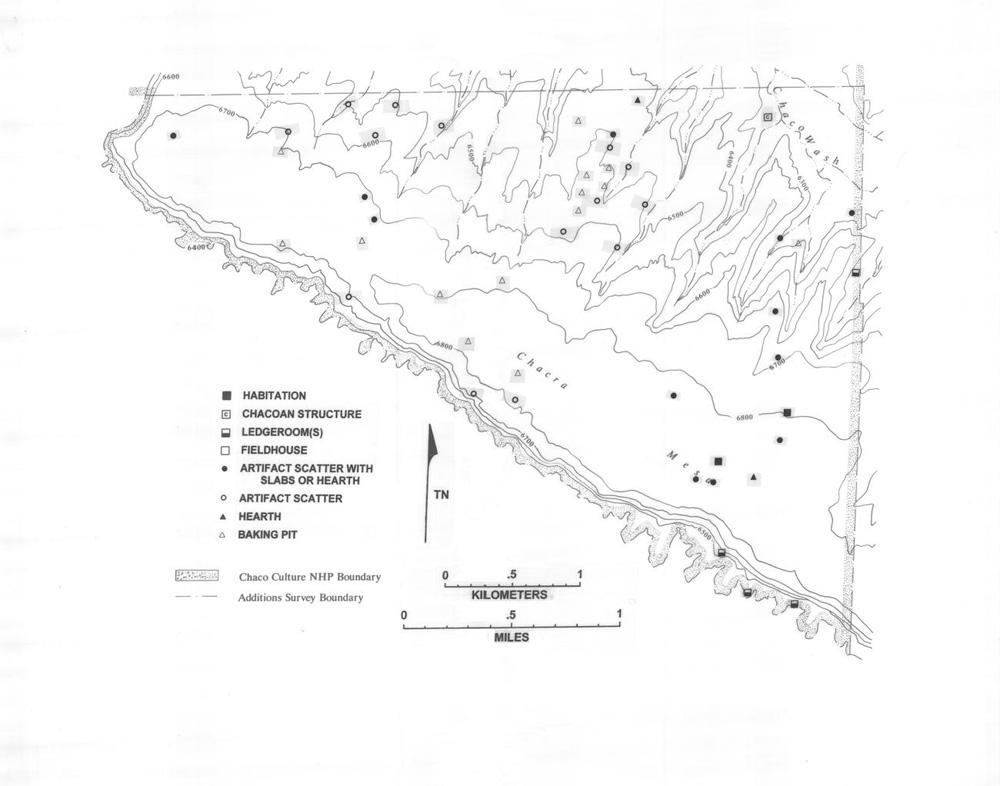Figure 2.30. Chacra Mesa survey area: A.D. 890-1025 (DG 300), A.D. 700-1025 (DG 250), and A.D. 890-1130 (DG 350) sites. Total components = 49.

¶ 112   Residential use of the Chacra Mesa area between A.D. 1030 and 1130 (DG 400) is largely confined to the lower reaches of the arroyos draining the northeastern most portion of the survey area (Figure 2.31). The Chacoan structure at 29SJ 2384 was probably occupied at this time and may have contributed to the formation of this habitation cluster. A few other habitation components also occur on the mesa top and along its southern edge near the eastern boundary of the survey area. A series of fieldhouse and ledgeroom components appear at the upper ends of several of the north-flowing drainages at this time, and the number of components in the western half of the survey area (all of them nonresidential and most of them nonstructural as well) reaches its maximum extent.

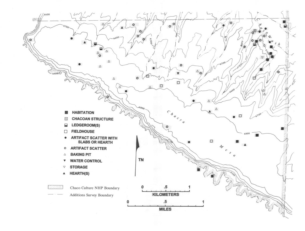Figure 2.31. Chacra Mesa survey area: A.D. 1030-1130 (DG 400), A.D. 890-1130 (DG 350), and A.D. 1030-1230 (DG 450) sites. Total components = 74.

¶ 113   Once again between A.D. 1130 and 1230 (DG 500) the portion of Chacra Mesa lying in the survey area was largely abandoned (Figure 2.32). An isolated great kiva was built further up the drainage above the now abandoned Chacoan structure at 29SJ 2384, and a small cluster of sites including one habitation component was established along the east-central boundary of the survey area. Otherwise, occupation was extremely sparse, and the westernmost portion of the mesa was wholly abandoned.

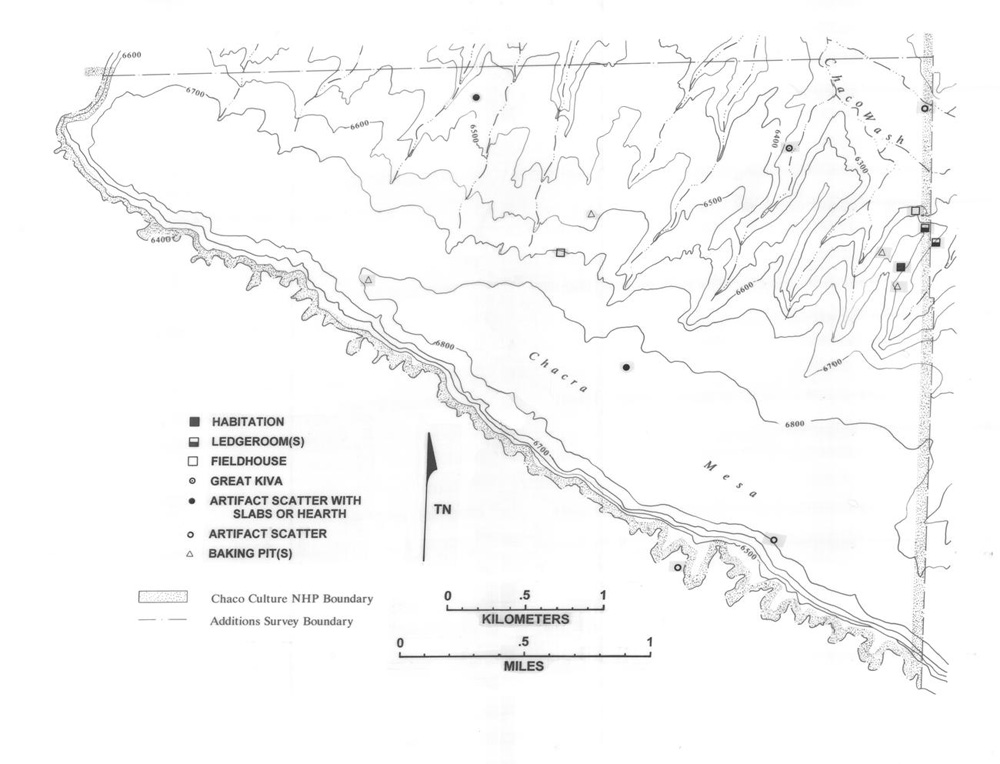Figure 2.32. Chacra Mesa survey area: A.D. 1130-1230 (DG 500) and A.D. 1030-1230 (DG 450) sites. Total components = 14.

¶ 114   The preceding discussion of the geographical distribution of settlement in the Chacra Mesa is based on dated components. The distributions of the largely undated, and often “unknown” in terms of cultural affiliation, water control, baking pit and hearth, rock art and shrine, and road/trail and associated components are of considerable interest, both relative to the settlement patterns shown in Figures 2.28 through 2.32 and in general.

¶ 115   The water control components66 [CLOSE]These include 9 Anasazi and 17 Unknown components. (Figure 2.33), for example, are distributed along the shallower north-flowing drainages at the western end of the mesa, a long way from the centers of habitation during all time periods in this area. The presence of fieldhouse and ledgeroom components at the heads of several of these drainages during the A.D. 1030 to 1130 (DG 400) period and of artifact scatter components on the margins of some others may indicate that this part of the survey area was being farmed seasonally by families maintaining residences outside the area during the A.D. 1030 to 1130 (DG 400) period. Another possibility, given that most of these water control components cannot be assigned even a cultural affiliation, is that these features pertain to the Navajo occupation of Chacra Mesa and were not part of the Anasazi settlement pattern at all.

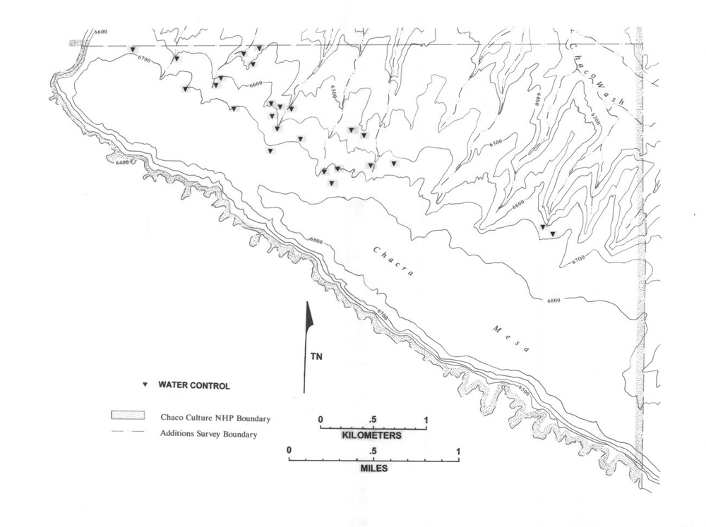Figure 2.33. Chacra Mesa water control components of Anasazi and Unknown cultural affiliation. Total components = 25.

¶ 116   The baking pit and hearth component map77 [CLOSE]The hearths include 1 Archaic, 13 Anasazi and 87 Unknown components. Baking pits include 1 Archaic, 57 Anasazi and 119 Unknown components. (Figure 2.34) presents a remarkable picture, especially when this map is compared with the corresponding maps for the other three survey areas. The large number of components of these types, their largely even distribution across the survey area, and the similarity of distribution of the two component types are all of interest.

¶ 117   At least two hypotheses may be offered to account for this concentration of baking pit and hearth sites in the Chacra Mesa survey area. The first is that some resource or resources found only in this part of the surveyed areas was being processed in the hearth and baking pit features at these sites. The second is that the heavy concentration of these components in the only surveyed area with an indigenous supply of firewood implies that whatever activities were carried out at these sites (for example firing pottery), it was more convenient to transport the needed supplies and equipment to Chacra Mesa than to transport the firewood used in these activities to a location closer to habitation sites.

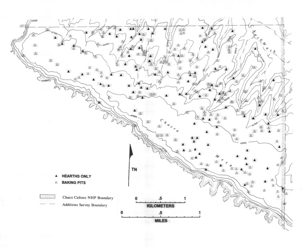Figure 2.34. All Chacra Mesa baking pit and hearth components of Anasazi and Unknown cultural affiliation. Total components = 278.

¶ 118   The largely even distribution of these components across the surveyed portion of Chacra Mesa would seem to offer an argument against the first hypothesis. If this hypothesis were true, we might expect a more clustered distribution of components in some particular environmental zone, but except for a slightly lower observed density in the area of dune activity in the very center of the mesa top, these components are ubiquitous throughout the survey area. The similarities in distribution between the component types could indicate a functional similarity or identity between baking pits and hearths. On the other hand, this similarity could be simply a function of a need for firewood as part of two distinct sets of activities.

¶ 119   The distribution of rock art panels88 [CLOSE]These include 4 Unknown and 63 Anasazi rock art components. (Figure 2.35) is, of course, related to the presence of suitable rock outcrops along the edges of the mesa. The heavy concentration of such panels in the northeastern portion of the survey area is probably also related to the long-term residential use of this area. Although none of the rock art components can be dated, it is interesting to note that the rincon with the greatest panel density in this northeastern area is the one that was the center of A.D. 1030 to 1130 (DG 400) habitation. The next drainage to the west, which was the locus of heavy A.D. 550 to 750 (DG 100) occupation, has far fewer rock art components. The density of panels along the southern margin of the mesa may be simply a reflection of an abundance of suitable rock faces in that area, but it could also be related to occupation of the area below the mesa edge, which was outside the survey area. There are only three Anasazi shrine components in the Chacra Mesa survey area (Figure 2.35). All three consist of single or paired C-shaped structures with low masonry walls, and all appear to be located with respect to vantage points. One is on the north edge of the mesa; one is on the south edge; and one is on the southwestern most tip of the mesa.

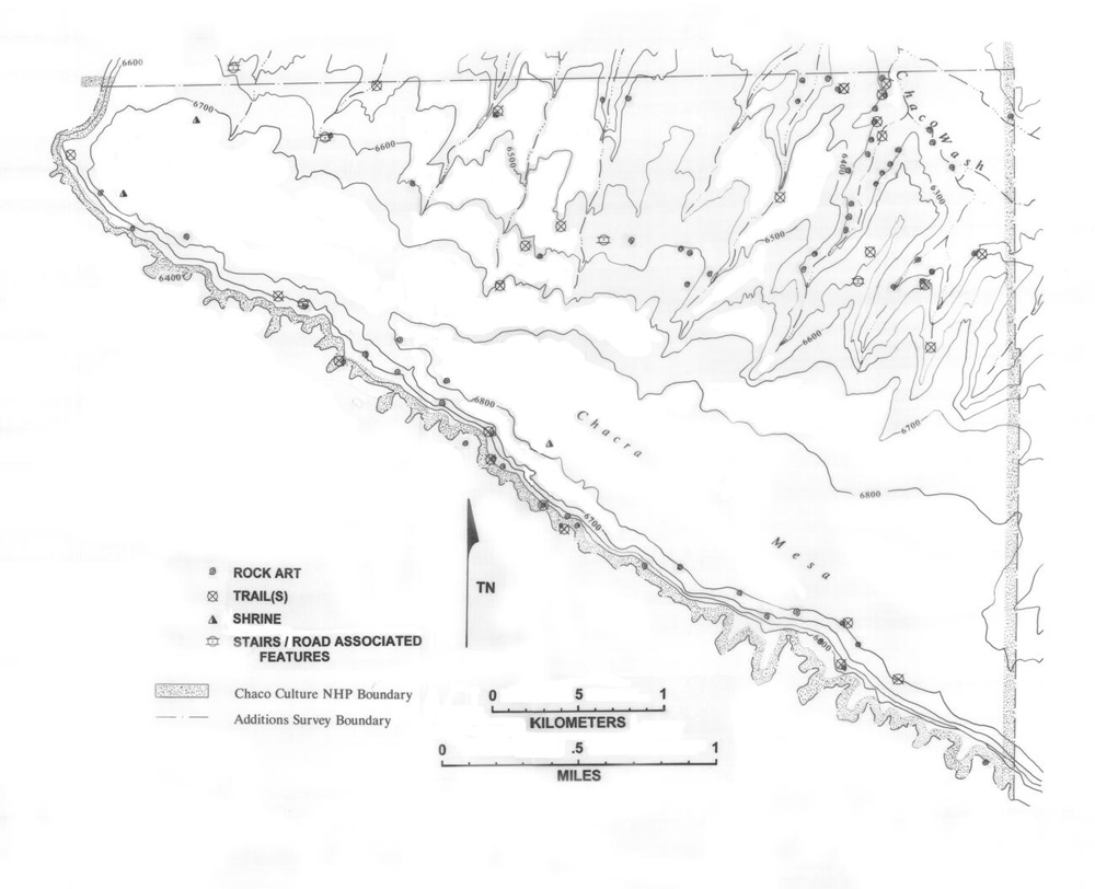Figure 2.35. All Chacra Mesa rock art, shrine, trail, and stairs/road associated components of Anasazi and Unknown cultural affiliation. Total components = 99.

¶ 120   The locations of road/trail segments and stairs99 [CLOSE]There are 20 Anasazi and 5 Unknown road/trail components and 4 Anasazi and 1 Unknown stair components. in the Chacra Mesa survey area (Figure 2.35), like those of rock art panels are conditioned to a large extent by topographic factors. These components occur along north flowing drainages leading up to the mesa top and at breaks in the south face of the mesa. One very interesting feature of this distribution is its similarity to the distribution of rock art. While topographic variables are certainly implicated in this similarity, by no means are all possible locations for components of either type occupied; the correspondence between rock art locations and road/trail locations appears to be more than coincidental. Of the 22 multicomponent sites in the Chacra Mesa survey area that included a road/trail component, 14 or 63.6 percent also included a rock art component, and this does not take into account proximity of components of these types that were defined as separate sites.

South Addition

¶ 121   Figures 2.36 through 2.39 illustrate the distribution of component types by date group in the South Addition [Note that there were no A.D. 1130 to 1230 (DG 500) components in this survey area]. Figure 2.40 shows the distribution of the water control, baking pit, hearth, shrine, rock art, and road/trail and associated components.1010 [CLOSE]There are 6 Anasazi and 2 Unknown rock art components, 2 Anasazi road/trail components, 3 Unknown baking pit components, 1 Anasazi and 1 Unknown hearth components, 1 Anasazi and 1 Unknown watercontrol components. Because this survey area is so small and because its boundaries are purely artificial relative to cultural developments in the Chaco Canyon area during the Anasazi period, it is difficult to do more than briefly characterize the settlement distribution; the meaning of the observed patterns is impossible to assess without information about settlement patterns in the surrounding areas.

¶ 122   Figure 2.36 shows that the A.D. 550 to 750 (DG 100) settlement of this survey area consisted of a small number of habitation and artifact scatter components located on the lower slopes to the southwest and southeast of South Mesa. Figure 2.37 shows that in this area, as in Kin Klizhin and especially on Chacra Mesa, A.D. 700 to 880 (DG 200) was a time of decreased occupational intensity. Three habitation components in the southeastern portion of the survey area and an isolated storage component on the slopes of South Mesa constitute the entire settlement system for this period.

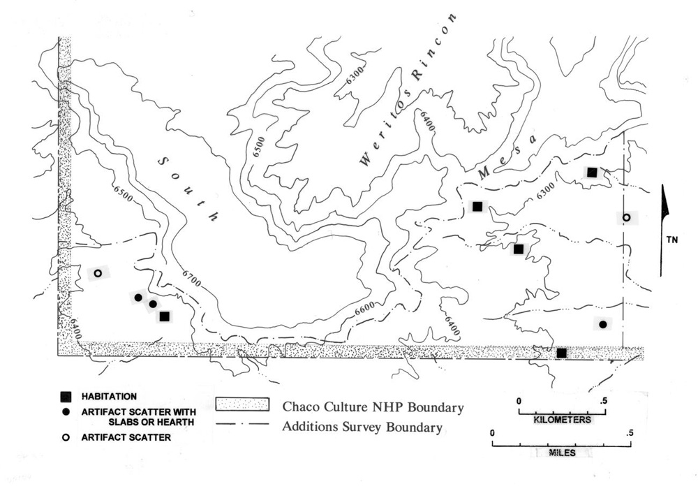Figure 2.36. South Addition survey area: A.D. 550-750 (DG 100) sites. Total components = 10.

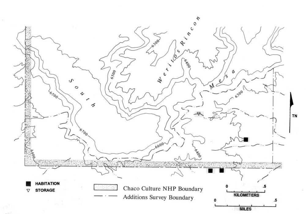Figure 2.37. South Addition survey area: A.D. 700-880 (DG 200) and A.D. 700-1025 (DG 250) sites. Total components = 4.

¶ 123   Occupational intensity increased markedly between A.D. 890 and 1025 (DG 300), at least in the southeastern portion of the survey area (Figure 2.38), and this occupation increasingly took the form of nonresidential use. Fieldhouses and artifact scatters constitute a significant portion of the settlement system at this time. Between A.D. 1030 and 1130 (DG 400) (Figure 2.39), the number of components is actually less than between A.D. 890 and 1025 (DG 300), although the distribution remains similar and the shift to nonresidential use continues.

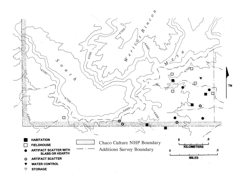Figure 2.38. South Addition survey area: A.D. 890-1025 (DG 300) and A.D. 700-1025 (DG 250) sites. Total components = 21.

Figure 2.39. South Addition survey area: A.D. 1030-1130 (DG 400) sites. Total components = 14.

¶ 124   Preserved water control features are extremely rare in this area. The two extant examples are located in a single east-flowing drainage (Figure 2.40). With the exception of one hearth, all baking pit and hearth components are distributed along the southeast slopes of South Mesa at roughly the same elevation (Figure 2.40). Rock art panels along the perimeter of South Mesa (Figure 2.40) do not exhibit any particular correspondence with the location of habitation components of any time period or in general. The single recorded trail segment (Figure 2.40) does, however, occur in conjunction with a rock art component.

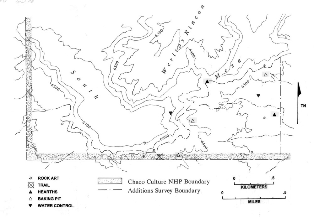Figure 2.40. All South Addition rock art, road/trail, baking pit, hearth, and water control components of Anasazi and Unknown cultural affiliation. Total components = 17.

Site Typology Evaluation

¶ 125   The site typology portion of this research had two goals. The first was to determine whether the site types, as defined in the field, and the component types derived from these site types in the course of the analysis were indicative of any measurable variability other than the variability in presence/absence of features on which these types were based. Were components of a particular type more likely to be similar to each other and different from components of other types in terms of artifact assemblages or temporal or spatial distribution? The second goal was to identify potential functional data relevant to the various site types and their suggested functions.

Evaluation of Component Types

¶ 126   As noted in the section on computerizing the data, where possible the site type assigned during the survey determined the component type assigned during the analysis. When new component types had to be assigned, the same morphological criteria used to determine site types in the field (Chapter 1) were applied. The only exceptions were the artifact scatter with hearth and artifact scatter with slabs component types, which were combinations of two field types.

¶ 127   Because these site/component types were assigned on the basis of presence/absence of features, assessment of their validity had to be based on other classes of data in order to avoid circularity. We adopted three approaches. The first involved an examination of variability within and between component types in artifact assemblages. The second approach involved an examination of the proportions of different component types over time and across space, as well as an examination of component type distributions, both geographic and in relation to environmental zones. The third approach involved a computer-assisted cluster analysis. In this third analysis individual components were grouped into clusters based on proportions of different ceramic wares and vessel forms in their artifact assemblages. These clusters were then examined to determine the component type breakdown of their constituent components.

Component Type Comparisons

¶ 128   The first step in assessing the site typology was to examine the success of the criteria used in dividing sites into unambiguous categories. The first logical bifurcation in classifying sites found during this survey can be based on the criterion of structural versus nonstructural. Ignoring for the moment the problem of surface visibility, this decision point should create two mutually exclusive classes, but in fact there are some uncertain types in the typology as it now exists. The clearly structural types are habitation, fieldhouse, ledgeroom, Chacoan structure, and great kiva. The clearly nonstructural types are all the scatters (sherd, sherd and lithic, lithic, scatter with slabs, and scatter with hearth), hearths, baking pits, water control, road/trail, stairs, and rock art.

¶ 129   The remaining component types are ambiguous. The cist/storage category is ambiguous because it lumps isolated storage rooms with small cists; even if it could be argued that these two feature types were both used for storage, the major differences in capacity of these two feature types make it unlikely that they could be considered functionally equivalent. This type, therefore, not only lumps structural and nonstructural components together, by definition it lumps two dissimilar features together in a way that is likely to mask considerable functional variability. The creation of an “isolated cist” component type in the nonstructural category and of an “isolated room” component type in the structural category would solve this problem of lumping together very dissimilar sites.

¶ 130   The shrine and road associated (herradura) categories are troubling because they have no specific identification criteria. Shrines are described as “ceremonial or other apparently esoteric sites,” and both types are described as including low-walled, circular, or C-shaped enclosures. A single descriptive type called “enclosure” or “rock alignment/enclosure” would be more generally applicable and would not require such specific functional assessments in the field.

¶ 131   The structural component types as defined are relatively straightforward and can generally be divided into mutually exclusive categories based on the criteria provided in the field manual. Habitation components were defined on the basis of the presence of surface structures of more than two rooms or of pitstructures or both. Fieldhouses were defined as having two or fewer rooms per surface structure and no pitstructures. Chacoan structures were identified on the basis of distinctive masonry, room size, mound height, site plan, and/or association with great kiva or road features. Ledgerooms were defined on the basis of their topographic setting.

¶ 132   Although these criteria permit the formation of mutually exclusive groups, some of them appear arbitrary. The use of the “two rooms or less/two rooms or more” criterion to separate fieldhouses from habitations, for example, could benefit from documentation, as could the assumption that pithouses are not used as fieldhouses (cf. Sebastian 1983, 1985). Additionally, the decision to lump all sites with residential structures of any form together into a single “habitation” category not only puts sites with very different sets of features into the same group, but as discussed in the data summary section, combines sites with very different temporal distributions and artifact assemblages as well.

¶ 133   In general, the nonstructural types are based on specific descriptive characteristics that identify particular kinds of variability (a sherd scatter versus a sherd and lithic scatter, for example) and thus it is fairly easy to assign sites unambiguously to a single type. The combined category of road/trail, however, lumps two distinct types of features together in a way that probably masks significant variability, and they might best be made into two separate types.

¶ 134   In the course of the computer coding process a problem having to do not with the site typology but with feature types was identified. The only designated feature type available for concentrations of rock was the “slab/fire-cracked rock scatter” category. This meant that concentrations of rubble, fire-cracked rock, burned slabs, and even burial slabs had to be coded as the same feature type. Because concentrations of rock of one sort or another were among the most commonly recorded features, assignment of all these concentrations to a single feature type masked a good deal of variability. By the time we realized the magnitude of the problem, it was too late to go back and separate construction elements into burned and unburned and both from piles of fire-cracked rock, although we did create a separate feature type for burial slabs. In future analyses, use of a wider variety of feature type designations for rock concentrations would probably be informative.

¶ 135   The spatial, temporal, and artifactual patterning of the various component types has already been outlined in the data summary section; only some of the observations worth emphasizing will be repeated here. Table 2.9 demonstrates that the relationship between the proportion of plainwares and the total proportion of jars in an assemblage is more complex than might be expected. Both the plain/decorated portion and the bowl/jar proportion within the decorated ceramics must be taken into account in characterizing any ceramic assemblage. It was these attributes that were used in running the cluster analysis described below.

¶ 136   Table 2.10 indicates that the distribution of trachyte-tempered ceramics and other imported wares is not the same across the component types. To an extent, this pattern is a result of temporal effects—other imports peak between A.D. 1130 and 1230 (DG 500) while trachyte wares peak between A.D. 1030 and 1130 (DG 400). But even if we control for time and look only at A.D. 1030 to 1130 (DG 400) components, for example, Chacoan structures still have the highest proportion of trachyte and a much lower proportion of other imports than habitations, fieldhouses, and scatter with hearth components.

¶ 137   Likewise the observation that fieldhouses have a higher proportion of trachyte ceramics than habitations at first glance seems attributable to the higher proportion of very early [A.D. 550 to 750 (DG 100)] components among the habitations. If the two component types are compared with time held constant, however (Table 2.21), fieldhouses still have a higher proportion of trachyte in the A.D. 550-750, 700-880 and 1030-1130 time groups than contemporaneous habitations. Indeed, during the A.D. 1030 to 1130 (DG 400) period fieldhouses have a trachyte proportion that is as high as or higher than the proportions at Chacoan structures (compare Table 2.21 and Table 2.14). This observation raises some interesting questions about the relationships among fieldhouses, Chacoan structures, and habitations. It is unfortunate that so few assemblages from Chacoan structures were available for this analysis; this one observation appears to suggest that many of the fieldhouse components may have been occupied by groups or individuals with close associations with the Chacoan structures.

¶ 138   Many of the differences among pithouse only, roomblock only, and combined pithouse/roomblock components have already been mentioned. In addition to the marked temporal patterning of these different habitation subtypes, two other arguments having to do with changes in site organization and site function can be offered for recording habitation sites in terms of these subtypes. As noted in the site data summary section, roomblock only components recorded during the survey have three times as many kivas and possible kivas as the roomblock/pithouse components. This observation, combined with the observation that certain other feature types such as baking pits are differentially represented on the different subtypes, would indicate differences in the organization of both sacred and secular activities among the habitation subtypes.

¶ 139   The other argument for preserving the distinctions among the subtypes has to do with the information presented in Tables 2.15 and 2.16. The shift from a settlement system dominated by habitation components in the early periods [39 percent of all components between A.D. 550 and 750 (DG 100) are habitations; 47 percent are habitation between A.D. 700 and 880 (DG 200)] to a system comprising a wide variety and large number of other component types [only 14 percent of A.D. 890 to 1025 (DG 300) components and 23 percent of A.D. 1030 to 1130 (DG 400) components are habitations] indicates that the organization of land use and the functional place of habitation components in the settlement system changed greatly over time.

¶ 140   Simply put, one would expect that many of the activities represented by the various nonhabitation component types in the later time periods were performed at the habitations during the earlier periods. The increasing size of roomblocks over time (Tables 2.18 and 2.19) and the increasing clustering of habitations into communities (Figures 2.12 through 2.16, 2.20 through 2.24, 2.28 through 2.32, and 2.36 through 2.39) are other aspects of this same pattern. As habitation sites became larger and more clustered, more activities were performed at loci distant from the habitation, creating a settlement system containing many sites of narrow or specialized function and a series of habitations that also exhibited a narrower range of activities.

The Cluster Analysis

¶ 141   A cluster analysis is a technique that involves comparing individual members of a group of objects or observations with one another and arranging them into clusters of individuals such that the clusters are as internally homogeneous and as externally heterogeneous as possible. Clusters can be disjoint, which means that each individual is assigned to only one cluster, or hierarchical, which means that one or more clusters can be included within a larger cluster. Although disjoint clusters are more often used when the goal is developing a typology, hierarchical clusters are also useful because they can indicate “family resemblances” among types.

¶ 142   We ran both types of clustering algorithms on the survey data using the proportions of plainware, decorated bowls, and decorated jars in the assemblage for each component as the variables on which the clusters were to be formed. We chose these particular variables in order to make this analysis consistent with a similar analysis performed as part of the ceramic research. We eliminated components of type “other” and “unknown,” as well as any component with fewer than 20 sherds from this analysis. We used the CLUSTER procedure from SAS (Ray 1982), which forms hierarchical clusters, to provide a TREE diagram showing the numbers of clusters that we could expect. From this we concluded that between 10 and 20 clusters would be interpretable without masking too much of the variation.

¶ 143   To derive the disjoint clusters against which to compare the results of the component type classification we used the FASTCLUS procedure in SAS, which allows the researcher to specify a desired number of clusters. We first ran FASTCLUS for 20 and 10 clusters. The 20-cluster analysis proved to be less than informative. More than half of the clusters contained very small numbers of cases—eight contained three or less. In addition, the large number of clusters meant that the distance between clusters was small (or the similarity between neighboring clusters was high), and this in turn meant that even the most cohesive component types were spread over a number of clusters, making the results somewhat difficult to interpret.

¶ 144   The 10-cluster analysis (Table 2.23) was more successful. Only two of the ten clusters were in the one-to-two cases range, although three others contained only five or six cases. The elimination of multiple closely related clusters also meant that the distribution of component types among the clusters was easier to discern and compare. Given that half of the clusters still contained very small numbers of cases, however, and that even the major component types were still generally spread over two to four clusters, we made an additional FASTCLUS run, specifying five clusters.

Table 2.23. Results of cluster analysis for ten clusters.

¶ 145   The 5-cluster analysis (Table 2.24) reduced the number of very small clusters to one and reduced the variability in cluster membership for some component types (e.g., fieldhouses), but by no means for all (e.g., roomblock-only habitations). The important observation here is that even with only five clusters, there is no component type (or at least none with more than one analyzed component!) whose members occur only in one cluster. One possible explanation for this pattern is that the site/component types classify only the variability in activities at a site that is reflected as presence/absence of features. The variability in activities that is reflected in the make-up of the ceramic assemblage, it might be argued, cross-cuts the variability that is reflected in features. Certainly much of the multicluster distribution of various component types that we see in Tables 2.23 and 2.24 could be a result of cross-cutting activity sets. The concentration of the majority of components of the feature-based type “pithouse only” in one ceramics-based cluster and of the feature-based type “roomblock only” in two different ceramic-based clusters, however, shows that at least in some cases activity variability of both kinds coincides.

Table 2.24. Results of cluster analysis for five clusters.
Component Type	Cluster No.					Total
	1	2	3	4	5
Pithouse	0	26	0	1	1	28
Pithouse/roomblock	0	28	0	5	10	43
Roomblock	0	12	0	18	21	51
Fieldhouse	1	26	0	8	22	57
Ledgeroom	0	7	0	5	11	23
Ceramic scatter	4	14	0	4	9	31
Ceramic and lithic scatter	1	5	0	5	9	20
Hearth	0	1	0	0	1	2
Baking pit	2	11	0	3	9	25
Water control	0	1	0	3	4	8
Cist/storage	0	0	0	1	2	3
Shrine	1	2	1	1	1	6
Great kiva	0	0	0	1	0	1
Chacoan structure	0	3	0	1	1	5
Road/trail	0	1	0	2	3	6
Scatter with slabs	0	15	0	4	11	30
Scatter with hearth	1	24	1	2	14	42
TOTAL	10	176	2	64	129	381
	Cluster Means	Plainware	Decorated Bowls	Decorated Jars
	1	11.6	4.3	84.0
	2	82.1	8.3	9.6
	3	0.0	91.0	9.0
	4	53.2	27.4	19.4
	5	50.6	14.3	35.1

¶ 146   This difference between the temporally differentiated habitation component subtypes points to the other major source of explanation for the multicluster distribution of most component types. Even a cursory examination of Table 2.21 indicates that within each component type, there are significant changes in the proportions of the three ceramic variables over time. Fieldhouse ceramic assemblages, for example, range from a mean of 91.2 percent plainware in A.D. 550 to 750 (DG 100) to 54.9 percent plainware in A.D. 1130 to 1230 (DG 500). Other component types exhibit similar temporal variability. It is hardly to be expected, therefore, that all components of a single type would fall into the same cluster, even if feature-based and ceramic-based typologies were measuring exactly the same variability in activities.

¶ 147   The logical solution to this problem of temporal variability within component types would be to run the cluster analysis again, this time comparing only components of a single date group. Unfortunately, the number of components in the sample is simply not large enough to permit date group by date group analysis. As Tables 2.23 and 2.24 show, eliminating “other” and “unknown” components and those components with fewer than 20 recorded sherds reduced the sample from 730 to 381 components. Given the relative proportions of the total number of components that fall in each date group and assuming that the “other,” “unknown,” and “too small” components are proportionately distributed, we could expect only 37 components of all types in a A.D. 550 to 750 (DG 100) cluster analysis sample, or 19 in a A.D. 700 to 880 (DG 200) sample, or 14 in a A.D. 1130 to 1230 (DG 500) sample. Even A.D. 1030 to 1130 (DG 400) would have only 103 components among all 17 types.

¶ 148   In an effort to assess the effect of this temporal variability on the relationship between component types and ceramic clusters, we examined the fieldhouse components, the largest group of components remaining once the habitations had been divided into subtypes. These fieldhouse components were first divided into date groups, and then the components from each time period were compared with the cluster means for the 10-cluster and 5-cluster analyses. This process was carried out by hand, so the results are only approximately comparable with the results of the computer analysis. Nevertheless, the results proved to be very interesting and more complex than anticipated.

¶ 149   All fieldhouse components with the required minimum number of sherds in their assemblages in A.D. 550 to 750 (DG 100) and A.D. 700 to 880 (DG 200) samples fell into Cluster 6 of the 10-cluster analysis and Cluster 2 of the 5-cluster analysis. The early fieldhouse assemblages uniformly are dominated by plainwares, with fewer than 10 percent (in A.D. 550 to 750; DG 100) or 20 percent (in A.D. 700 to 880; DG 200) decorated sherds.

¶ 150   The A.D. 890 to 1025 (DG 300) fieldhouse assemblages were found to encompass a great deal of variability. Of the 14 assemblages from this period, seven fell into Cluster 9, three into Cluster 6, and two each into Clusters 5 and 10. Relative to the 5-cluster groupings, there were six in Cluster 2, five in Cluster 5, and three in Cluster 4. What this indicates is that during this period there are at least three general types of fieldhouse assemblages. There are still a number of components with heavy representations of plainware, but there are even more components with plainwares in the 60 to 70 percent range, the difference being made up by an increase in decorated jars. At the same time, there are also several components with less than 60 percent plainware and a decorated assemblage dominated by bowls rather than jars.

¶ 151   The A.D. 1030 to 1130 (DG 400) assemblages exhibit somewhat less variability, but they do not fall into a single cluster using either set of cluster means. Instead, most of the components—17 out of 25 for the 10-cluster analysis and 22 out of 25 for the 5-cluster analysis—fall into two clusters, Clusters 7 (n=8) and 9 (n=9) in the first case and Clusters 2 (n=8) and 5 (n=14) in the second. Two of the three exceptions in the 5-cluster case are very small assemblages (fewer than 30 sherds); the third is a Cluster 4 assemblage. The exceptions in the 10-cluster case include four assemblages that fall into Cluster 10; three of the remaining exceptions are very small assemblages, while the fourth is a large assemblage that falls into Cluster 6.

¶ 152   This breakdown indicates the majority of A.D. 1030 to 1130 (DG 400) fieldhouses exhibit one of two types of ceramic assemblages—an assemblage with roughly between 55 and 70 percent plainwares and a decorated assemblage dominated by jar forms or an assemblage containing 40 to 50 percent plainwares but with a decorated assemblage also dominated by jars. A smaller number of components exhibit a plainware percentage somewhere between those of the main clusters and have a decorated assemblage dominated by bowl forms. The A.D. 1130 to 1230 (DG 500) fieldhouse assemblages appear to exhibit at least as much variability as the A.D. 890 to 1025 (DG 300) assemblages. There are only five components from this time group in the sample, but in the 10-cluster scheme one is Cluster 4, one is Cluster 6, one is Cluster 7, and two are Cluster 9.

¶ 153   The results of this time period by time period examination of the fieldhouse assemblages clearly indicates that a great deal of temporal variability is affecting the distributions of components into clusters shown in Tables 2.23 and 2.24. The differences among the three habitation subtypes that can be observed in these tables also indicates the strong influence of temporal variability on the ceramic attributes being used to form the clusters and assign components to them. For this reason, it is impossible to say how internally homogeneous and externally heterogeneous the component types are (relative to the ceramic variables being monitored) or to suggest possible functional differences and similarities among the types based on this cluster analysis. A similar analysis using a larger sample that would permit controlling for time, however, could prove to be very informative about both the cohesiveness of the types and relationships among types.

Functional Implications

¶ 154   In evaluating the functional implications of the site typology used during the survey, it is important to point out that these site types mix purely descriptive terms (e.g., “ceramic and lithic scatter”) with terms indicating general function (e.g., baking pit) and terms denoting rather specific functions (e.g., fieldhouse). In all cases, however, field identification of site types was based purely on morphological data. This final section of the site typology evaluation will offer assessments of the functions ascribed to the function-specific site types and suggestions about possible functions for the descriptive site types.

Habitations

¶ 155   The term habitation refers simply to a place where people live. In archaeology this term is generally used in the sense of a “residence.” The term is used to imply a relatively sedentary, long-term (that is, more than a few days or weeks) occupation and generally supposes the presence of shelters and a wide range of domestic and maintenance activities. For addressing some types of archeological questions—notably those concerned with demography—it is important to determine whether habitations were occupied year-round or seasonally abandoned, but for purposes of site typology, habitations can be defined as the main residence of the occupants.

¶ 156   Most Anasazi habitation sites appear to have been occupied during the colder parts of the year (Sebastian 1983). They exhibit such thermal properties as contiguous structures or subterranean structures, substantial walls, small doorways, and interior hearths and/or heating pits. They generally also contain ample storage space for the food supplies needed during the winter and provide sheltered facilities for performing chores often done outside during mild weather (e.g., cooking, grinding, weaving). Habitation sites occupied year-round could be expected to exhibit all these features and to have multiple outdoor activity areas as well.

¶ 157   The artifact assemblage at a habitation site should contain items indicating the full range of domestic activities—processing, storage, preparation, and consumption of food; manufacture of tools, utensils, and furnishings; social and religious activities; craft and leisure activities. Even at year-round habitations, and more especially at seasonally occupied habitations, many economic activities (e.g., farming or hunting) would be expected to take place away from the residence.

¶ 158   All habitation components in the survey sample contain, by definition, substantial, thermally efficient residential structures. This component type has one of the largest mean component sizes (Table 2.6), indicating either longer term occupation or a greater variety of activities (or both) than at most other component types. The ceramic assemblage from the habitations contains a high proportion of plainware jars, indicating storage and cooking activities, and a high proportion of bowls among the decorated assemblage, indicating food preparation and serving (Table 2.7). The lithic tool types recovered from habitations (Table 2.8) indicate a wide range of both on-site activities (e.g., corn grinding) and maintenance activities (e.g., broken projectile points).

¶ 159   Differences among the three habitation subtypes cast an interesting light on the question of year-round versus seasonally occupied habitations. Data on the numbers of the various component types recorded for each date group (Table 2.15) indicate that while a large proportion of the sites in the early date groups were habitations [39 percent in A.D. 550 to 750 (DG 100), 47 percent in A.D. 700 to 880 (DG 200)] sites of this type constitute a much smaller proportion of the settlement system during later periods [14 percent in A.D. 890 to 1025 (DG 300), 23 percent in A.D. 1030 to 1130 (DG 400), 19 percent in A.D. 1130 to 1230 (DG 500)]. This change in the pattern of occupation would seem to indicate that increasing numbers of tasks were being performed at some distance from the habitation sites by individuals or groups who established temporary residential sites or at least used single loci often enough or intensively enough to leave recognizable traces (sites) in the archeological record.

¶ 160   This change in the settlement system occurred simultaneously with the shift from pithouse to roomblock habitations; 82 percent of the pithouse-only habitation components date to A.D. 550 to 750 (DG 100), A.D. 700 to 880 (DG 200) and A.D. 700-1025 (DG 250), while 91 percent of the roomblock-only components date to A.D. 890 to 1025 (DG 300), A.D. 1030 to 1130 (DG 400), A.D. 1030-1230 (DG 450) and A.D. 1130 to 1230 (DG 500) time groups (Table 2.17). We would expect, therefore, that pithouse-only components would be more likely to be occupied year-round and that many roomblock-only components may have been abandoned for at least part of the agricultural season.

¶ 161   Two pieces of information from the survey analysis, neither of them conclusive, seem to support this suggestion. The first is that habitation component mean size is much larger in the Chacra Mesa survey area than in the other areas (Table 2.13); because Chacra Mesa has by far the largest proportion of pithouse only habitation components, this suggests that pithouse sites are, on average, larger than roomblock-only sites. Although inter-pithouse spacing may affect site size, the small average number of pithouse features (1.1 pithouses and 1.8 possible pithouses) per pithouse component argues against attributing this size difference wholly to necessary separation of the subterranean structures.

¶ 162   Generally site size is a function of a) number of occupants or b) length of occupation. If we consider one pithouse to equal one domestic unit and three roomblock rooms to equal one domestic unit, the averages of fewer than three pithouses and of 7.8 surface rooms per habitation component would indicate similar population sizes for both pithouse only and roomblock only habitations. This suggests that it is variability in period of occupation that is causing the differences in site size: either pithouse sites were occupied longer in terms of number of years per site or they were occupied for a longer portion of each year or both.

¶ 163   The other potential indicator of year-round habitation on the pithouse sites is the mean number of features per component. Pithouse components have more than twice as many features per component as roomblock-only components (or half again as many features if Shabik’eshchee Village is excluded from the sample). This is especially striking because the pithouse only components are older than the roomblock sites, sometimes by several centuries, and therefore extramural features on the former have had a longer time to be covered or destroyed. Because features observable in a survey context are of necessity extramural, this greater number of features on pithouse sites would tend to indicate a greater intensity of warm season occupation.

Fieldhouses

¶ 164   Although the term fieldhouse is often used as if it referred to a unified phenomenon, the range of variability in sites that fit this broad functional definition is large. Moore (1979) has defined five different patterns of use for fieldhouses:

(1) daily, returning nightly or most nights to the habitation; (2) bi-seasonal, during the spring planting and the fall harvest; (3) late-seasonal, as the crop approaches maturity and during and shortly after the harvest; (4) sporadic, as fields and crops require attention; and (5) continual, more or less steadily throughout the agricultural season (1979:89).

¶ 165   Ethnographic studies and fieldwork conducted as part of the Navajo Mine Archeological Program (NMAP; Sebastian 1983) supported Moore’s suggested subtypes of fieldhouses. Continual or full-season fieldhouses were found to include substantial structures; a wide range of domestic trash, often deposited in localized middens; interior features for cooking and heating during inclement weather; and ethnobotanical evidence for utilization of wild plants available throughout much of the agricultural season.

¶ 166   Bi-seasonal and late seasonal fieldhouses tended to be less substantial structures, though still with interior thermal features; trash disposal was less concentrated, but still consisted of the full range of domestic refuse; ethnobotanical evidence was limited but was tentatively interpreted as indicating that some sites were occupied both during early summer and late summer while others were occupied late summer only.

¶ 167   Sporadic and day-use fieldhouses could not be separated analytically. Both appeared in the archeological record as components with no evidence of structures, with limited quantities of sheet trash, and with ceramic assemblages heavily dominated by jars, both plainwares and painted.

¶ 168   Based on the site type definition criteria used during the inventory survey and analysis, the components defined as fieldhouses are most likely to be full-season fieldhouses in the NMAP typology. The various fieldhouses used for only part of the agricultural season would most likely appear as scatter with slabs or scatter with hearth components, while the day-use fieldhouses are most likely classified as ceramic or ceramic and lithic scatters.

¶ 169   One of the most important things about fieldhouses other than day-use ones is that people live there. For this reason we would expect to find the full range of daily domestic trash on such sites. Day-use sites, on the other hand, would be heavily dominated by jars because little or no cooking took place at these sites and water containers would be the main ceramic vessels present there. Table 2.21 indicates that when the component-specific ceramic assemblages are controlled for time, fieldhouse assemblages are similar to those of habitations in all time periods.

¶ 170   What all this indicates is that habitations and fieldhouses will be very similar in terms of artifact assemblages. Most of the trash found on archeological sites is the result of daily domestic activities, and these activities tend to be the same whether the family is living in a 50-room pueblo or a 2-room fieldhouse. The functional differences between fieldhouses and habitations are most likely to be reflected as differences in component size, number and permanence of structures, degree of emphasis on storage, and importance of ritual, craft, and maintenance activities.

Scatters

¶ 171   It has been suggested above that scatter with features components, ceramic and lithic scatters, and ceramic scatter components might represent fieldhouses of decreasing degrees of permanence, with the ceramic scatters representing possible day-use sites. Table 2.21 shows that the scatter with hearth and scatter with slabs components exhibit the “domestic ceramic assemblage” pattern discussed for habitations and fieldhouses, with scatter with hearth components more closely resembling habitations and scatter with slabs components more closely resembling fieldhouses.

¶ 172   The ceramic and lithic scatters appear to be quite variable and do not closely resemble either habitation or fieldhouse assemblages. The ceramic scatters do have a higher proportion of jars in their decorated assemblages than the fieldhouse and habitation components, but they do not have higher proportions of plainwares as expected. Components of these two types are probably best interpreted as resulting from a number of different activities, including day trips to work in agricultural fields or to collect wild resources.

Ledgerooms

¶ 173   Ledgerooms are small structures or enclosures built against cliffs or outcrops at the top of talus slopes, against large boulders, or under overhangs or rockshelters. Some have two (but usually no more) contiguous rooms; more often multiroom components consist of several isolated structures. These rooms tend to be quite small—usually less than 2 by 2 meters—and at least those in overhangs are low-ceilinged—often 1 meter or even less. Most of the ledgeroom components (63.9 percent) are in the Kin Bineola or Chacra Mesa (33.3 percent) survey areas, and most of those that can be dated (16 of 25) are between A.D. 1030 and 1130 (DG 400).

¶ 174   Ledgeroom components take three forms. More than 30 percent of all ledgeroom components consist of structures with no or almost no associated artifacts. Around 40 percent of the ledgeroom components consist simply of the structures and associated artifact scatters, some of which are quite extensive or quite dense. The rest of the ledgeroom components consist of structures, artifact scatters, and additional extramural features—mostly hearths and baking pits.

¶ 175   Given the size, appearance, and setting of these features, it seemed likely that they would prove to be storage structures. The presence of numerous thermal features in association with ledgerooms, the numbers of artifacts present on some components, and the composition of the ceramic assemblages on those components with associated artifacts all argued against this interpretation, however.

¶ 176   Ledgerooms found in isolation, without associated artifacts or features, most likely are storage features. If all ledgerooms were purely storage features, however, the ceramic assemblages might be expected to be dominated by sherds of storage containers—plainware and decorated jars. In fact, assemblages from those ledgeroom components with ceramics contain only low to moderate proportions of plainwares and moderate proportions of bowls among the decorated wares (Tables 2.7 and 2.9).

¶ 177   While ledgerooms do not have as high a proportion of bowls among their ceramics as habitations or fieldhouses, they do have a much higher proportion of this vessel form than the cist/storage components (Tables 2.7). This, plus the presence of the numerous thermal features, indicates that at least some domestic activities were carried out in or around these structures—although relatively few could have been carried out in the structures, given their very small size. The project documented an unusually high proportion of decorated jars in the ledgerooms as compared with fieldhouses and habitations. This pattern merits further investigation.

¶ 178   The discovery of a cache of digging sticks and a possible carrying basket frame in a ledgeroom component on Chacra Mesa (29SJ 2577) offers an interesting perspective on these sites. Although nothing definite can be said about overall site function and season or intensity of occupation without excavation, currently available data permit us to make at least some suggestions about function. Ledgeroom components appear to have had a combined storage/limited domestic occupation function. Given their frequent location on points of vantage above potential farm fields, it seems likely that agricultural tools and supplies were cached in these locations convenient to the point of use; temporary storage of at least part of the harvested crops in these structures also seems a likely possibility.

¶ 179   With the arrival of each agricultural season, families or other work groups may have come to these structures, unsealed them and removed cached equipment and possibly reserve seed corn. As they prepared the fields, planted the crop, and remained at the field to protect the sprouting plants, the storage structure would have become a natural center for activities, given its sheltered location against a cliff or boulder and the availability of the structure for storing food and other perishables. Larger ledgerooms could even have served as temporary shelters during inclement weather.

¶ 180   As the agricultural season progressed, groups or individuals may have come to work in the fields on a day-use or sporadic basis, contributing to the higher jar proportion in the decorated ceramics by introducing water containers. The common occurrence of baking pits on ledgeroom components may indicate green corn consumption as part of the field site activities. With the harvest, tools and equipment would again have been cached in the ledgeroom, possibly along with extra seed corn. Some portion of the harvested crops may have been stored in the structure temporarily to be retrieved as needed during the winter. The structure would then have been sealed until the next spring.

¶ 181   Clearly much of this reconstruction of ledgeroom component function is conjectural, but it does conform to the known attributes and variability of components of this type. More intensive study, including excavations, of this little-known site type should be given priority in future plans for managing the cultural resources at Chaco Canyon.

Baking Pits and Hearths

¶ 182   The recommendation made at the end of the ledgeroom discussion applies even more strongly to the baking pit and hearth components. The sheer number of these thermal features and their wide-spread distribution, especially on Chacra Mesa (Figure 2.34), indicate that they constituted a ubiquitous feature of the land-use system, and yet without excavation data we have no means to determine what their function within that system was. Although these component types have similar spatial distributions and ceramic assemblages, the differences in temporal distribution, component size, and assemblage size between the two component types imply functional differences as well.

¶ 183   Clearly these features were used to heat something, but whether they were used in processing some wild plant resource, to roast green corn, to fire pottery, or for all of these purposes or some other use entirely is unknown. The concentration of these features on Chacra Mesa and their wide-spread distribution across that area would seem to indicate that they were located so as to take advantage of convenient firewood sources. If these features were used in processing wild plant resources, however, they may be located with respect to the distribution of this resource or resources.

¶ 184   Baking pit components were the fourth most common component type recorded during this survey; on Chacra Mesa they were the second most common type after rock art panels. No comprehensive statement about Anasazi land use in the Chaco Canyon area is possible without some functional information on these features.

Chacoan Structures and Great Kivas

¶ 185   This survey has provided invaluable information about the nature and distribution of sites in portions of the communities surrounding the Kin Klizhin and Kin Bineola outliers. These data are particularly useful for assessing change over time in such communities and for making comparisons between an early, potentially largely independent outlier system such as Kin Bineola and a late system with high potential for close ties to Chaco Canyon such as Kin Klizhin.

¶ 186   In terms of adding to our understanding of the function of Chacoan structure and great kiva components, however, the small sample and limited data recovery inherent in such a survey cannot be expected to compare with the results of major surveys of the outlier system (Marshall et al. 1979; Powers et al. 1983) or intensive excavations (Breternitz et al. 1982; Windes 1987). The ceramic data collected during the survey do offer some insight into the question of Chacoan structure function, however.

¶ 187   The ceramic analysis indicates that there are slight but noticeable differences between Chacoan structure assemblages and those from other contemporaneous sites (compare Chacoan structure assemblage statistics from Table 2.7 with the A.D. 1030 to 1130 (DG 400) statistics for other component types in Table 2.21). Chacoan structures are not simply large habitations; they have a considerably higher proportion of plainwares and therefore a lower proportion of decorated wares. Within the decorated wares they have a higher proportion of decorated jars (and thus a lower proportion of bowls). They also have somewhat more trachyte-tempered and other imported ceramics. Chacoan structures have a higher proportion of plainwares than any other A.D. 1030 to 1130 (DG 400) component type and a higher proportion of decorated jars than any of the A.D. 1030 to 1130 (DG 400) structural component types.

¶ 188    The meaning of these ceramic patterns is difficult to suggest with the present data (see Chapter 4 for comparisons with other Chacoan assemblages). Jars of both ware categories are commonly associated with storage; grayware jars were used extensively in cooking. With additional information on presence/absence of sooting and on orifice diameter of the vessels it might be possible to formulate some hypotheses about differences in activities between the Chacoan structures and contemporaneous small-site habitations.

Settlement Pattern Analysis

Methods

¶ 189   The inventory surveys concentrated on four non-contiguous areas. Two of these areas, Chacra Mesa and the South Addition, are best viewed as part-and-parcel of Chaco Canyon itself. The other two areas, Kin Klizhin and Kin Bineola, have been termed “outliers,” a designation that indicates the presence of a Chacoan structure and numerous sites clustered in a relatively discrete area.

¶ 190   The analysis of settlement patterns reported here takes into account this important difference between the outlier study areas and those adjacent to the canyon. For Chacra Mesa and the South Addition, any attempt to study the areas as though they were self-contained units would be misleading. Our approach has been to analyze the survey results from these areas in such a way that the results will be as comparable as possible with the Hayes (1981) survey of the main portion of the canyon. In contrast, Kin Bineola and Kin Klizhin were analyzed as self-contained units, even though the areas surveyed around Kin Bineola and Kin Klizhin did not encompass all sites in these outlier communities. The proportion of each community represented in the survey is unknown, and therefore the representativeness of the sample is difficult to gauge.

¶ 191   The spatial analysis of the survey data concentrated on three dimensions—time, function, and environment. Each of these dimensions was operationalized as a discrete variable. The temporal span was broken into the five date groups established by the ceramic analysis (Chapter 4). It is worth reiterating that some components could not be dated at all while others had components that spanned more than one date group. The assignment of functional component types has already been discussed.

¶ 192   The environment was categorized into 32 vegetative/geomorphic types (Chapter 3). Each unit of land in the four areas was classified into one and only one vegetative/geomorphic type. Likewise, each site was associated with only one of these environmental variables. This classification system allowed us to assess site location in relation to site-specific environmental variables, that is, to determine whether more sites or fewer sites than expected by chance are located in each environmental zone. We cannot, however, determine how sites are situated in relation to surrounding catchment zones with the present automated data. To do so we would need to return to the vegetative/geomorphic map, draw a catchment zone of a specified radius (e.g., 250 or 500 meters) around each site, and then calculate the area represented by each zone found in the catchment circle. Such an endeavor is possible with the available data, but the process is extremely time-consuming and was beyond the scope of this project. Thus with the present data, we can say that a site was located on good agricultural land but not how much of this land. Further, the number of sites located on poor agricultural land can be determined, but we cannot tell whether these sites are close to or far from potential agricultural fields.

¶ 193   Trends in settlement for all four areas were analyzed primarily through a series of contingency tables. For each area we first cross-tabulated environmental variables by component type. This gross tabulation was followed by the compilation of similar tables that indicated the numbers of component types by time period controlling for environmental zones. For example, for Kin Klizhin we produced a table that divided the 150 Anasazi components among the 19 component types and nine environmental zones represented in the survey area. For each environmental zone (e.g., uplands), all sites from the various component types were placed into the appropriate date group.

¶ 194   As an aid in this analysis, scatter plots were produced for each component type in each survey area. These plots were based on the UTMs recorded on the site forms. The scatter plots and contingency tables were produced using subroutines from version 9.0 of the Statistical Package for the Social Sciences (SPSS; Nie et al. 1985).

¶ 195   A second approach to studying settlement trends was applied to the outlier communities. In these cases, we were interested in not only the environmental context of sites, but also in their proximity to the Chacoan structure. Prior to conducting the analysis we suspected that the Chacoan structures would act as “magnets” and “pull” surrounding sites closer to them. We expected that sites would continue to be located in specific settings (e.g., near drainages), but that once the Chacoan structure was established sites would tend to cluster in those favored settings that were closest to the Chacoan structure. We also suspected that the Chacoan structures would exert different degrees of “pull” on different component types. Specifically, habitation sites might be drawn to the Chacoan structure, while fieldhouses and ledgerooms might not.

¶ 196   To test these expectations we computed the Euclidean distance between the Chacoan structures of Kin Klizhin and Kin Bineola and each component located in the surrounding survey area. For each component type we calculated the average distance from the Chacoan structure and the standard deviation. These calculations were performed by an SPSS subroutine.

Kin Klizhin

¶ 197   Tables 2.25 and 2.26 present the results of the settlement pattern analysis for Kin Klizhin. Somewhat surprisingly nearly half the Anasazi components are located in the uplands, which have a poor agricultural rating. In contrast, the lowland, dissected areas, which are some of the best agricultural land in the region, contained only one-third of the sites. The uplands constitute 233 ha (575 acres), or 43.1 percent of the surveyed area in Kin Klizhin, while the lowland, dissected regions encompasses about 210 ha (520 acres), or 39 percent. Thus, the uplands contained slightly more sites than would be expected by chance alone, whereas the lowland, dissected areas contained slightly fewer sites (neither relationship is very strong nor significant using a chi-quare test at an 0.05 alpha level).

Table 2.25. Kin Klizhin component types by vegetative/geomorphic zone.

Table 2.26. Distance in meters to Kin Klizhin Chacoan structure by component type and date group.

¶ 198   These overall trends are mirrored by the distribution of individual component types. The strongest individual trend is exhibited by habitation components, nearly 65 percent of which are found in upland settings and only 13 percent of which are found in lowland, dissected, areas.

¶ 199   At first glance the results appear counterintuitive. Examining the scatter plots of component distribution, however, indicates that nearly all habitations, fieldhouses, and scatters with features are located on the edge of elevated settings, overlooking the drainages. People may have been living in the uplands, but it is still likely that their agricultural fields were located just below, in, or near the drainages.

¶ 200   There is also evidence that the overall trends mask variation in settlement location through time. This is especially true for habitation sites. Of the 11 habitation sites dated between A.D. 500 and 1030, 10 were found in upland settings. Of the 11 habitation sites date between A.D. 1030 and 1130, however, only four were found in the uplands. The remainder were found in dissected lowlands (4), undissected lowlands (1), and badland outcrops (2).

¶ 201   This trend also applies to fieldhouses, but to a much lesser degree. Of the nine fieldhouses dated prior to A.D. 1030, five (55 percent) are found in the uplands, three (33.3 percent) in undissected lowlands, and one was found in the badland outcrops. Nineteen fieldhouses are dated to the period between A.D. 1030 and 1130. Of these, seven (36.8 percent) were found in the uplands, six (31.6 percent) in the dissected lowlands, and the remaining six were found scattered throughout several zones.

¶ 202   Shifts in preferred location are best shown graphically. The schematic maps in Figure 2.41a, b, c, d, and e show the locations of habitations and fieldhouses for A.D. 550 to 750 (DG 100) through A.D. 1130 to 1230 (DG 500) date groups. These figures are simplified versions of the ones presented in the Geographic Distribution section above. In this figure h represents the location of a habitation and f the location of a fieldhouse. Numbers indicate locations that contain more than one component.

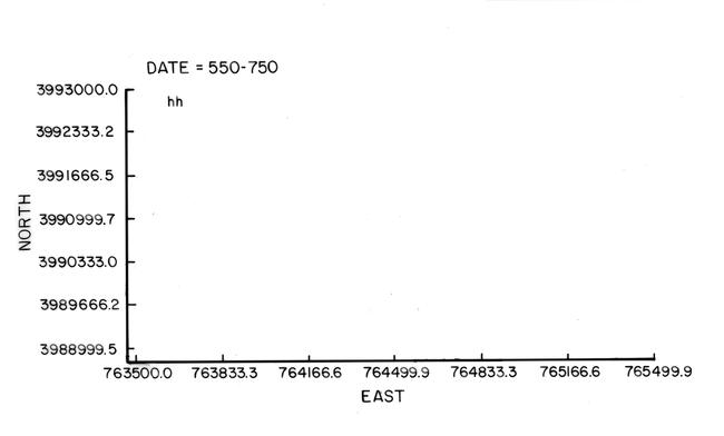Figure 2.41a. Habitation and fieldhouse distribution in the Kin Klizhin survey area, A.D. 550-750 (DG 100).

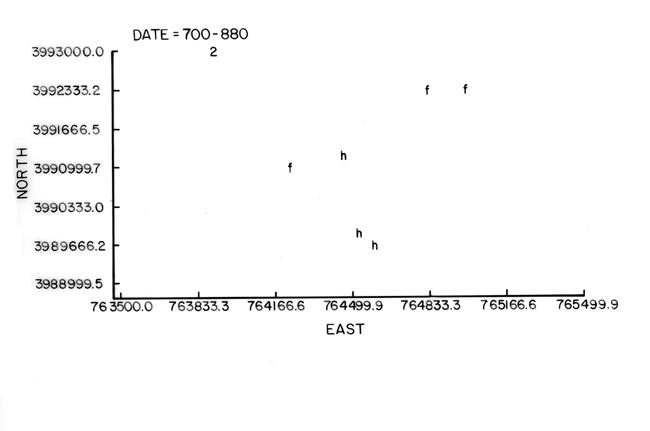Figure 2.41b. Habitation and fieldhouse distribution in the Kin Klizhin survey area, A.D. 700-880 (DG 200).

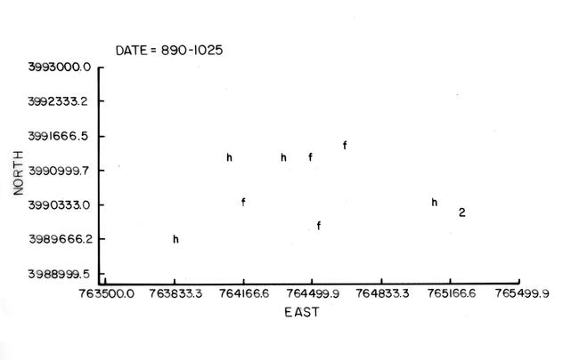Figure 2.41c. Habitation and fieldhouse distribution in the Kin Klizhin survey area, A.D. 890-1025 (DG 300).

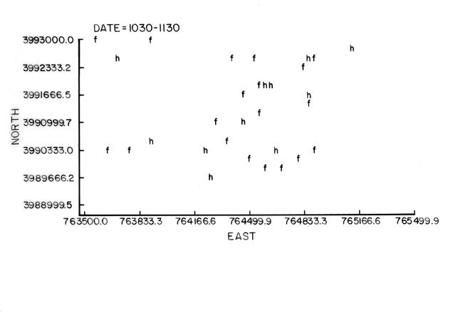Figure 2.41d. Habitation and fieldhouse distribution in the Kin Klizhin survey area, A.D. 1030-1130 (DG 400).

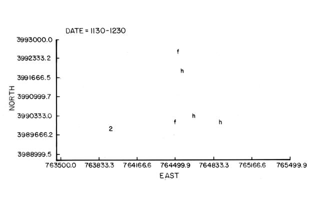Figure 2.41e. Habitation and fieldhouse distribution in the Kin Klizhin survey area, A.D. 1130-1230 (DG 500).

¶ 203   Figures 2.41a, b, and c show the general upstream movement (i.e. to the south) of habitation sites between A.D. 500 and 1030. Between A.D. 1030 and 1130 there is a general filling in of all arable land in the survey area which is followed by a major settlement collapse. While these shifts are interesting in and of themselves, perhaps the most important aspect of the settlement pattern is the relationship between habitation sites and fieldhouses.

¶ 204   Prior to A.D. 1030 fieldhouses were not extensively used. One possible explanation is that habitation sites were located on or near agricultural fields and that when cultivation shifted to new fields the habitation sites were moved as well. This could account for the general upstream movement of habitation sites and, presumably, of population. Between A.D. 1030 and 1130 habitation sites tend to be regularly spaced along all drainages, with fieldhouses interspersed between habitation sites. In terms of simple spatial relationships it appears that most of the habitation sites are associated with at least one and as many as four or five fieldhouses. This pattern would argue for some type of dispersed agriculture. Each habitation site may have been the locus of a social unit which was responsible for fields in two or more places.

¶ 205   If this scenario is correct, we would expect that habitation sites would be situated on or near the best agricultural land, and that the building of the Chacoan structure at Kin Klizhin would not have had a great effect on site location. This indeed appears to be the case, because as Table 2.26 indicates the establishment of Kin Klizhin did not exert a “pull” on other sites. Between A.D. 550 and 1025 habitation sites move closer to the area where the Chacoan structure would be established, but between A.D. 1030 and 1130, when Kin Klizhin was occupied, habitation sites and fieldhouses actually move farther away.

¶ 206   There is a danger in reading too much into these figures. The average shift in component type location is usually no more than 200 meters between date groups; that is, about 200 m in at least 100 years. Taking into account the standard deviations of the component distances, there are more overlaps in occupation between date groups than there are shifts. The basic trend at Kin Klizhin appears to be one of settling key areas and then moving around within these areas. This situation is consistent with the scenario outlined above: key areas containing the best agricultural land were settled first, with subsequent movement being a reflection of old fields becoming exhausted and new fields being established.

Kin Bineola

¶ 207   The surveyed area of Kin Bineola is divided primarily between two environmental zones; uplands, which encompass 141 ha (348 acres) or 26 percent of the area, and lowland, dissected regions, which constitute 234 ha (577 acres) or 43 percent of the region. Most of the sites are found in one of these two zones. Their proportioned distributions closely approximate the proportions of these zones in the natural environment, with 30 percent of the components being found in the uplands and 41 percent being found in lowland, dissected settings (Table 2.27). Only two other environmental zones have substantial numbers of components. These are the sandstone or shale outcrops which encompass 6.6 percent of the survey area and host 7.7 percent of the components, and the slopes, which cover 5 percent of the area and contain 9.4 percent of the components.

Table 2.27. Kin Bineola component types by vegetative/geomorphic zone.

¶ 208   Slightly over half of the habitation sites are found in the uplands, whereas most other component types are located in the lowland, dissected areas. There is a tendency through time for component location to change from upland to lowland, dissected settings. Overall this tendency is rather weak. Among habitation components, however, the shift from predominantly upland to lowland settings is relatively distinct. In the periods A.D. 500 to 750, 700 to 880, and 890 to 1025, the percentages of habitation sites in the uplands are 50.0 percent, 63.6 percent, and 66.7 percent, respectively. The percentage of upland habitation sites drops to 42.1 percent during the period from A.D. 1030 to 1130. In contrast dissected lowland settings, which prior to A.D. 1025 had averaged about 8 percent per date group, increased to 42.1 percent (or the same percentage as upland settings) during the period from A.D. 1030 to 1130. This trend also appears to characterize other component types. Due to the small numbers of components dated to each date group, one cannot place much confidence in these trends.

¶ 209   An examination of the data on mean distances from the Kin Bineola Chacoan structure or great house for the various component types reveals that habitation sites move away from the great house location through time (Table 2.28). This trend is graphically illustrated in Figures 2.42a, b, c, d, and e for fieldhouses and habitation components. Slow movement upstream in settlement is indicated. This pattern is not so much one of abandonment of downstream locations as it is of movement in the relative concentration of habitations. This pattern may be related to agricultural practices. It is also possible that the presence of a small Chacoan structure in the southern portion of the study area influenced the settlement pattern.

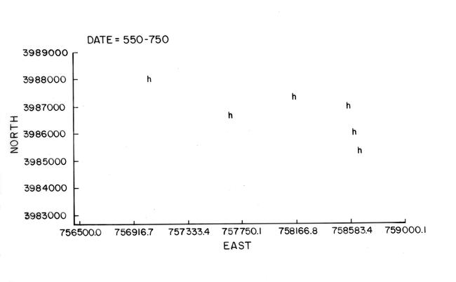Figure 2.42a. Habitation and fieldhouse distribution in the Kin Bineola survey area, A.D. 550-750 (DG 100).

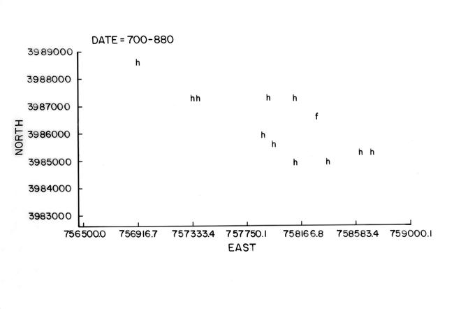Figure 2.42b. Habitation and fieldhouse distribution in the Kin Bineola survey area, A.D. 700-880 (DG 200).

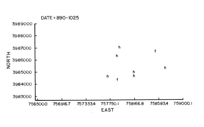Figure 2.42c. Habitation and fieldhouse distribution in the Kin Bineola survey area, A.D. 890-1025 (DG 300).

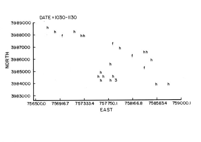Figure 2.42d. Habitation and fieldhouse distribution in the Kin Bineola survey area, A.D. 1030-1130 (DG 400).

Figure 2.42e. Habitation and fieldhouse distribution in the Kin Bineola survey area, A.D. 1130-1230 (DG 500).

Table 2.28. Distance in meters to Kin Bineola Chacoan structure (29SJ 1580) by component type and date group.

¶ 210   It is worth pointing out that the relationship between habitation sites and fieldhouses in Kin Bineola is very different from that which characterizes Kin Klizhin. In the Kin Klizhin survey area the ratio of habitation sites to fieldhouses during the period from A.D. 1030 to 1130 is 1:1.9, whereas for the same period in Kin Bineola the ration is 1:0.3. Clearly there was a major difference in the ways that the occupants of these areas related to their immediate environments. In Kin Klizhin the pattern suggests small dispersed agricultural fields, perhaps consistent with floodwater or akchin farming practices. At Kin Bineola the absence of fieldhouses and the tendency for habitations to occur in clusters suggests that another pattern was operating. One possibility is that the use of water control for farming was more important, perhaps favoring habitation in clusters as opposed to a dispersed pattern. The differences described above may have led to very different demographic patterns, a subject discussed in a later section of this chapter.

Chacra Mesa

¶ 211   Of the 21 environmental zones represented on Chacra Mesa six account for about 82 percent of the land area. These are, in order of decreasing abundance, bench, dissected, with sandy soil outcrops (37.5 percent); mesa outcrop-talus (12.7 percent); upland-rough dune (10.7 percent); cliff wall-talus (8.8 percent); upland loamy soils (7 percent); and overgrazed upland loamy soils (5.3 percent). These same environmental zones also account for nearly 90 percent of the Anasazi components recorded on Chacra Mesa (Table 2.29). Benches are the most heavily utilized zone, with over half (52.4 percent) of all Anasazi components being found in this zone. This trend is especially noticeable for baking pit components, which are the most frequently encountered archeological resource on Chacra Mesa. More than 67 percent of all baking pit components are located on benches. Although the distribution of resources is intriguing, it is not significantly different from what would be expected from a random process. The distribution of baking pits on benches versus their distribution on all other environmental zones yields a chi-square of 2.65, which with 1 degree of freedom has a p value of slightly more than 0.10.

Table 2.29. Chacra Mesa component types by vegetative/geomorphic zone.

¶ 212   Other component types that are found predominantly on benches are ceramic scatters (71.1 percent) and water control features (96.2 percent). The former are found throughout the Chacra Mesa survey area, while the latter are located almost exclusively in the western half. Water control features as a rule are not associated with either habitation structures or fieldhouses. It is possible that many of these features are Navajo in origin.

¶ 213   Not surprisingly most rock art is found in either the Mesa Outcrop-Talus or Cliff Wall-Talus zone. The Cliff Wall-Talus zone was also favored for the placement of ledgerooms and storage components.

¶ 214   Most component types show little evidence of shifts in environmental or geographic setting through time. Two major exceptions are baking pits and habitations. Of the 40 baking pit components that can be dated, 36 fall into one of three date groups: A.D. 550 to 750 (DG 100) (n=8), A.D. 890 to 1025 (DG 300) (n=14), and A.D. 1030 to 1130 (DG 400) (n=14). Of the A.D. 550 to 750 (DG 100) baking pit components, 62.5 percent occur on benches, a figure comparable to the percentage of all bench components dated to this period (56.1 percent). During A.D. 890 to 1025 (DG 300) the preference for benches as baking pit sites appears to have been more pronounced; 71.4 percent of baking pit components are found in this zone, as compared with 54.8 percent of bench components of all types. Finally, 78.6 percent of A.D. 1030 to 1130 (DG 400) baking pits are located on benches while only 58.3 percent of all components are located in this zone.

¶ 215   Habitations are found primarily in the highly dissected northeastern quarter of the survey area. Sixty percent of the A.D. 550 to 750 (DG 100) habitation components are located on benches in this area. The numbers of recorded A.D. 700 to 880 (DG 200) and A.D. 890 to 1025 (DG 300) habitations are too small to permit any meaningful assessment of location. Of the 12 known A.D. 1030 to 1130 (DG 400) habitations, only one is located on a bench. The others are located in upland (2), lowland (3), slope (2), and outcrop settings (4) of various types.

¶ 216   This shift in preferred settings for habitations seems to be more apparent than real. An examination of Figures 2.28 through 2.32 shows that the real shift was a move from one drainage to another. The early occupation was clustered near the head of a deeply incised drainage that runs west of the promontory capped by Shabik'eshchee Village. The later occupation was centered along two drainages to the east. Thus while site specific environment locations differ, the overall environmental situation of Anasazi habitation components in the Chacra Mesa survey area remains approximately the same through time.

South Addition

¶ 217   In general the proportional distribution of sites among environmental zones in the South Addition does not closely mirror the percentages of the major zones in the survey area. An exception is the badlands and dissected hills with thin soils zone which encompasses about one-third of the total survey area and where nearly one-third of the components recorded were found (Table 2.30). Nearly one-third of the components recorded in this zone were habitation sites, and one-third or more of the majority of other component types were also located here. In a contrasting vein, 20 percent of the components were located in the Mesa Outcrop-Talus zone, which constitutes only 13.4 percent of the survey area. At first glance this result is surprising because this zone is rated as having poor agricultural potential. This seeming inconsistency is partially explained, however, because 40 percent of the components in this zone are rock art panels.

Table 2.30. South Addition component types by vegetative/geomorphic zone.

¶ 218   Finally, only 23 percent of the components were found in lowlands and drainages, which constitute 31 percent of the area and are classified as fair and good agricultural lands. This low percentage is misleading, however, because by definition percentages must sum to 100. Because so many rock art sites were found along the mesa outcrops, the percentages of all other zones are mechanically decreased. The point is that the lowlands and drainages in the South Addition were not less intensively utilized than those in other survey areas; in point of fact, 50 percent of the fieldhouses, sherd and lithic scatters, and scatter with slab components were located in this zone.

¶ 219   Temporal shifts are difficult to detect. Through time habitation sites that can be dated show a shift from badlands and dissected hills to lowlands. Because only 12 components can be dated, however, this tendency is tenuous at best.

Settlement Conclusions

¶ 220   Perhaps the most surprising aspect of the settlement pattern analysis was the lack of correlation between site location and particular environment zones. In none of the four areas were significant associations observed. This does not mean that settlement was random. Rather it implies that the manner in which the environment was measured does not reflect the way that the environment was perceived by the Anasazi occupants. One major problem is that the environmental analysis is site specific. That is, we know that sites are located in a particular environmental setting but know nothing about the surrounding zone. For example, analysis showed that the habitation sites in Kin Klizhin are located in upland areas with poor agriculture potential; with the data at hand there is no way to determine whether the “effective” environment of these sites includes areas where agriculture could have been practiced. While such an analysis is possible, it would require data not currently available.

¶ 221   Substantive results were obtained concerning settlement at the two outlier communities. In both cases the construction of a Chacoan structure does not appear to have greatly affected already established patterns of settlement. Subsequent movement appears to have been in response to microregional shifts in agricultural potential and not to have been greatly affected by social forces related to the larger Chacoan cultural phenomenon. This finding has implications for other outlier studies especially those for communities where settlement was established prior to the Chacoan structure. The Kin Bineola and Kin Klizhin results indicate that the constituent members of these outlier communities were concerned first with their own well-being and only secondarily with aspects of the greater society.

¶ 222   While tentative, these results are intriguing for they suggest something less than a tightly integrated society. If this scenario has merit, it raises a number of interesting questions. How were established settlement clusters integrated with the Chacoan structures? What did the occupants of these great houses have to offer established local communities? Were Chacoan outliers established in locations having to do with larger societal objectives with little concern for local networks? These are a few of the questions that the data from Kin Klizhin and Kin Bineola bring into sharper focus.

Demographic Analysis

Methods

¶ 223   Of all analytic topics in archeology, few are as problematic as the study of prehistoric demography. Population dynamics are assessed on the basis of assumptions whose validity is extremely difficult to evaluate. To complicate the issue, changes in population size and composition are often viewed as causally related to changes in other aspects of culture. In reading previous demographic studies concerning Chaco Canyon, one has the uneasy feeling that the population estimate flowed from a particular theoretical stance as opposed to the other way around. For example, some investigators have argued that population increase was a major cause of the development and florescence of the Chacoan culture (Altschul 1978; Grebinger 1973; Judge et al. 1981; Vivian 1970, 1974). These studies tend to emphasize those estimates that show a rapid population increase during a relatively short period of time and suggest a total population for Chaco Canyon at its height of between 4,500 and 6,000 people. Other investigators have pointed out that a population of this size could not have been supported by local resources alone (Schelberg 1982, 1984; Windes 1984). They suggest that a population size in the range of 2,000 to 3,500 people is more in line with the evidence.

¶ 224   The problem here is not so much that one set of estimates is right and the other wrong (although one would assume that this is the case) as much as it is our inability to evaluate any estimate. All the population estimates for Chaco Canyon follow logically from the set of assumptions upon which they are based. For the most part each investigator develops some type of function that equates numbers of people with observable attributes of the archaeological record. Hayes (1981:49-50) assumed that three rooms translated into 4.5 people. Windes (1984:83) used a function that equated one hearth with six people. Other transference functions have equated a set number of people with each kiva (Steward 1937) or with a given number of acres of arable land (Cully et al. 1982).

¶ 225   With some trepidation we offer yet another population estimate, be it only for the four inventoried areas. Given the range in variability of previous estimates, we feel it is incumbent upon us to be clear about the assumptions upon which the analysis is based. Before we offer these assumptions, however, it is important to emphasize certain points about the nature of the database. Our population estimates by necessity are based on sizes of features determined from surface observations. Only those feature types that were believed to be inhabited were used. These were features coded as roomblocks, Chacoan structures, pithouses, and possible pitstructures. The size estimates are as exact as was possible under field conditions, but their detail and accuracy are variable. For a Chacoan structure we often know its surface extent, and in some cases, the number of rooms. For less well defined features, such as surface scatters coded as habitations, the surveyors were able to record only the maximum extent of surface material.

¶ 226   Many problems exist with using site area based on surface indicators to estimate population (Hassan 1978, 1981). Surface scatters are generally larger than their corresponding subsurface deposits. In this situation, functions based on structure size are apt to yield misleading results, and our estimates are probably high. Unfortunately, we are not in a position to say how high; given the nature of survey data, however, there is really no way around this problem.

¶ 227   Previous population estimates for Chaco Canyon can be divided into two types. The first are those that focus exclusively on the Chacoan structures. These include the pioneering studies of Fisher (1934) and Pierson (1949) as well as the more recent work of Drager (1976) and Windes (1984). The second type of estimate is more regional in scope and includes data from both villages and Chacoan structures. Studies of this type are Schelberg (1982), Hayes (1981), and Cully et al. (1982).

¶ 228   Our analysis will be of the second type. It differs from previous estimates primarily in the particular demographic weighting factors applied to the different component types. For example, in Hayes’ (1981) estimates all rooms are equal, so that no matter whether it is located in a village or a Chacoan structure every group of three rooms is equated with 4.5 people. In this scheme Chacoan structures are viewed simply as scaled-up villages. This approach may be valid for periods prior to A.D. 950, but after that time this view of settlement may be misleading. Using data from the SJBRUS database, Judge (1983) and Gillespie and Powers (1983) have demonstrated that the San Juan Basin as a whole witnessed a nearly 300 percent increase in the number of habitation sites during Pueblo II (A.D. 900 to 1000). This growth rate is phenomenal. Using a simple function of equating X number of people with Y area of living space, we can show that such an increase would imply a population growth rate that simply could not have occurred through natural fertility.

¶ 229   At the time of the Chaco Additions survey, the authors deliberated between two possible explanations for this dramatic increase in site numbers: in-migration, or a shift to a more dispersed seasonal settlement pattern. Over the past decade, subsequent work has strengthened the former explanation. It appears likely that hundreds of residents from north of the San Juan River moved south into the Chaco region following the ninth century breakup of large, aggregated communities such as McPhee Village (see for example Van Dyke 2007, Chapter 4; Wilshusen and Van Dyke 2006; Windes n.d; Windes and Van Dyke 2012. for discussions). However, the authors’ original analyses are presented here as written in the 1980s.

¶ 230   In 1988, the authors considered that the dramatic increase in habitation sites between A.D. 900 and 1150, while almost certainly indicating some increase in population, may not reflect an increase of the magnitude that simple numbers suggest. The question, then, is how to model the demographics of this time period. We have opted for a staged approach. First, we calculated population for each time group using Naroll’s (1962) frequently applied formula

P=A/10

¶ 231   where P equals population and A is the area in square meters of the ith habitation feature. Areas were determined in the field for all features with the exception of most of the pithouses and possible pitstructures. In order to include these in the calculations, we used data provided in McKenna (1984:381) that show that the mean size of pithouses excavated in Chaco Canyon is 11.56 square meters. Using this mean figure, we estimated the habitable area of pithouse components by multiplying the total number of pitstructures by 11.56.

¶ 232   Although Naroll’s formula is easy to use, it is not without problems (Hassan 1978, 1981; LeBlanc 1971; Wiessner 1974). Drager (1976) fit Naroll’s formula to the demographic data of modern pueblos and argued that the fit was rather good. An examination of his results (Drager 1976: Figure 1), however, reveals that the relationship between area and population for the modern pueblos is not linear. As pueblo size increases, population also increases but at a progressively slower rate. Using the modern pueblo data provided by Drager (1976) and Stubbs (1950) we reanalyzed the relationship between occupation area under roof and population. The results, shown in Table 2.31 and shown graphically in Figure 2.43, indicate that a power regression of the formula

y=0.17456x0.90827

¶ 233   has the highest associated r value (0.767), which is a substantial improvement over the 0.574 r value for the linear regression.

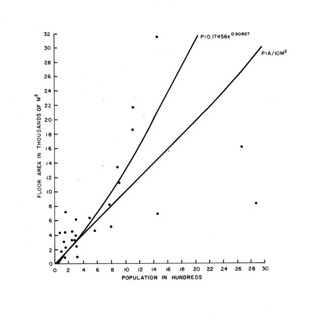Figure 2.43. Relationship of population to area under roof for modern pueblos using a linear regression and power regression model (adapted from Drager 1976: 163).

Table 2.31. Population and area under roof, modern Pueblos.

¶ 234   In the second phase of the demographic analysis, we calculated the population of each of the four surveyed areas using the power regression formula derived from modern pueblo demographic data. This approach may be realistic for above-ground pueblo data, but we found that it did not work very well with pithouse data. In part this is a result of basing our pithouse size estimate on excavations in the canyon. The excavated pithouses tend to be late and are all associated with above-ground structures. Earlier pithouses were larger, presumably to allow for storage space that was later moved to the above-ground structures. The net result is that population estimates for A.D. 550 to 750 (DG 100) and A.D. 700 to 880 (DG 200), which are based primarily on pithouse data, appear to be too low.

¶ 235   To compensate we recalculated our estimates using an arbitrary figure of five people per pithouse. Thus, to determine the population of a pithouse component we simply multiplied the number of actual and possible pithouses by five. For other features, population was derived using the power regression formula. In the results section this method is referred to as the “power+” estimation method.

¶ 236   Even the power+ approach is not without problems. The most serious complication concerns sites with both pithouses and surface structures that date to the same period. Most of these sites date to the A.D. 700 to 880 (DG 200) era. Based on current evidence, it seems likely that the pithouses and surface structures were occupied by the same group at the same time. By including both features in our population estimate we are in effect double counting. To alleviate this problem we made separate population estimates, using the power+ method, for roomblocks and for pithouses and possible pitstructures on components with both types of habitation structures. We then used only the higher population estimate of the two to represent that component. For example, site 29SJ 2490 in Kin Klizhin has an estimated population of 14 people based on surface structures and 15 people based on the three pithouses present; we estimated the component population as 15, which is the higher of the two possible estimates. We refer to this approach as the “power+ adjusted” method.

¶ 237   The approaches described thus far assume that a feature was occupied to its maximum potential for each time period represented. For a single-component site this causes no problems, but for multicomponent sites, this assumption is unrealistic, especially for the large Chacoan structures. For example, Kin Bineola has an estimated population of 480 using Naroll’s formula, 380 using the power regression, and 391 using either the power+ or power+ adjusted methods. Because this site was occupied during both the A.D. 890 to 1025 (DG 300) and A.D. 1030 to 1130 (DG 400) periods, these figures are entered in the population estimates of both periods.

¶ 238   There are a variety of methods that could have been used to alleviate this situation. We could have divided the population evenly between the two date groups, or we could have allocated the population proportionally between the date groups using as a weighting factor the proportion of sherds dated to each time period. We originally intended to use the latter approach but did not have the necessary ceramic data.

¶ 239   In the absence of a reliable means of modeling population at multicomponent sites, we chose not to divide the population estimates at all. Our figures, then, can be viewed as maximum population estimates. That is, the estimates represent the upward limits of population at any one time. The population almost assuredly never reached these limits, but it is not clear how close it came.

¶ 240   The factors affecting our population estimates are not likely to have had as severe an effect on estimates of growth rates. Unless it can be demonstrated that sites in one date group have larger or smaller surface scatters for the same number of inhabitants, the growth rate, which essentially compares the amount of “habitable” area from one period to another, should not be greatly affected. For this reason we emphasize these rates over the actual population figures in the results section. Growth rates were calculated using the formula

r = [ln(N) – ln(N0)] / t

¶ 241   where ln is the natural logarithm and ln(e) equals 1, r is the rate of population growth, the population for a date group is N0, N is the population for the succeeding date group, and t is the number of years in the period. The time period was calculated by representing each date group by its midpoint. Date group 100 which extends between A.D. 550 and 750 was assigned A.D. 650, date group 200 (A.D. 750-890) was assigned A.D. 820; date group 300 (A.D. 890-1030) was assigned A.D. 960; date group 400 (A.D. 1030-1130) was assigned A.D. 1080, and date group 500 (A.D. 1130-1230) was assigned A.D. 1180.1111 [CLOSE]For the purpose of estimating population the time period ranges were adjusted to eliminate overlaps and gaps between periods. See Table 2.2 for comparison. Intervals between date group midpoints were: date group 100-200 170 years; date group 200-300 140 years; date group 300-400 120 years; date group 400-500 100 years.

¶ 242   Although our estimates are simple and comparable, this does not necessarily mean that they are accurate. In a final attempt to model population as accurately as possible we added another assumption that we feel is justified although we are aware that other Chacoan scholars might not agree.

¶ 243   Basically, we assumed that much of the population maintained residency at both the Chacoan structures and at habitation sites located nearby. This is not to suggest that Chacoan structures were empty ceremonial structures occupied only on specific occasions or that all members of a social group moved into and out of the Chacoan structure seasonally in a rigid, mechanical pattern. We suspect that the occupational dynamic was much more complex. Small groups would have maintained ties to a Chacoan structure and with one another while pursuing essentially subsistence agriculture.

¶ 244   The apparent paradox of semiautonomous units existing in the context of a larger cohesive social entity is not as problematic as it may seem. The ability to fragment society has adaptive advantages in a marginal environment. An aggregated population offers increased potential for pooling and redistribution of resources and for cooperation in other ways, but organizationally and socially it is clearly a more difficult pattern to sustain than a pattern of autonomous domestic units. Tension between individual social groups and the larger community is a common theme in pueblo ethnography, and what has been viewed as disintegration may actually be a very powerful adaptive stance (e.g., Eggan 1950, French 1948, Titiev 1944).

¶ 245   Regardless of the social implications, the suggested pattern of dual residence has clear demographic implications. If this assumption is correct, by including both habitation sites and Chacoan structures in the population estimates, we would be in effect double counting. To circumvent this problem we could either subtract the Chacoan structures or the other habitation sites from the population estimates. We chose to eliminate the former because with few exceptions the latter were occupied during only one date group, thereby eliminating the problem of multicomponent sites discussed above. One problem with this approach is that many of the small habitation sites probably were not occupied for a full date group. The estimates, therefore, may be somewhat high, although the error should be consistent for each date group.

Results

¶ 246   The results of the demographic analysis are presented in Tables 2.32 and 2.33 and graphically displayed in Figures 2.44 and 2.45; the raw data used in this analysis are presented in Appendix 2.4. Population reached its zenith in the Kin Klizhin, Kin Bineola, and South Addition survey areas between A.D. 1030 and 1130 (DG 400). Chacra Mesa, with its large Basketmaker III community centered around Shabik'eshchee Village, has its highest population during the A.D. 550-750 (DG 100) period, although population rebounds during the A.D. 1030-1130 (DG 400) interval. Maximum possible population estimates during the A.D. 1030-1130 period range from 317 to 348 for Kin Klizhin, 1,190 to 1,343 for Kin Bineola, 394-415 for Chacra Mesa, and 96 to 104 for the South Addition (Table 2.32). More realistic maximum population estimates, excluding the Chacoan structures, are between 137 and 166 for Kin Klizhin, 756 to 808 for Kin Bineola, and 335 and 353 for Chacra Mesa for the A.D. 1030-1130 period. The South Addition maximums are unchanged since this area has no Chacoan structure. At this point a comparison of these results with figures based on agricultural output alone may be of interest.

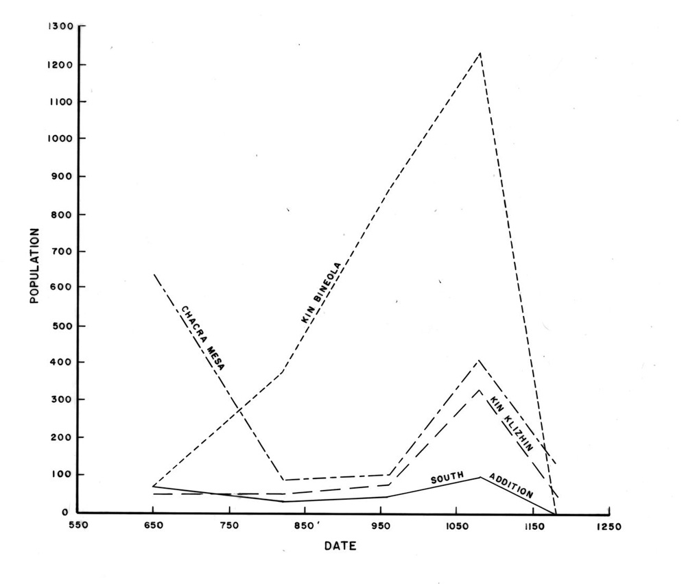Figure 2.44. Population trends using Power + adjusted formula, maximum estimates. Population during each period has been plotted at the period midpoint.

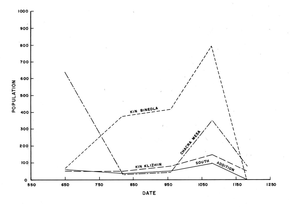Figure 2.45. Population trends using Power + adjusted formula minus Chacoan structures. Population during each period has been plotted at the period midpoint.

Table 2.32. Population estimate totals.

¶ 247   Using data from ethnographic studies of Navajo floodwater farming in the Bis sa'ani area, Cully et al. (1982) estimated that it takes about 0.81 to 1.214 ha or two to three acres of arable land to support one person. These figures probably can be applied to the present survey areas with little difficulty. By combining the hectares of good and fair agricultural land (as defined by Cully and Toll in Chapter 3) in each of the survey areas and then dividing by 0.81 and 1.214 ha, maximum population figures for groups depending on floodwater farming can be derived. Using this method, we find that 214 to 321 people could have been supported in the Kin Klizhin study area, 265-398 people in Kin Bineola, 173-259 on Chacra Mesa, and 52-78 in the South Addition (see Table 3.5). The estimates for Chacra Mesa and the South Addition are difficult to evaluate because these areas cannot be considered to have been independent of Chaco Canyon. The figure for Kin Klizhin corresponds fairly well with our estimates for this area, but the estimate for Kin Bineola is one third to one half of our estimated population maximum.

¶ 248   We believe that differences in settlement patterns in the Kin Klizhin and Kin Bineola areas discussed earlier point to a possible explanation of the differing results of these two population estimating procedures. As noted in the settlement pattern discussion, in Kin Klizhin habitation sites are regularly spaced and often are associated with multiple fieldhouses. This pattern is suggestive of a system dependent on floodwater farming, and the congruence between our population estimate and the estimate based on floodwater farming agricultural potential would seem to support this suggestion.

¶ 249   In the Kin Bineola survey area, on the other hand, habitation sites are clustered and there is a much lower ratio of fieldhouses to habitations. This pattern suggests that there may have been more cooperation between habitation units, with perhaps proportionately less land being worked. This situation is not consistent with agriculture based on floodwater farming, but it is congruent with more intensive practices that utilize some form of water control, and such intensive systems can support a larger population than systems based on floodwater farming.

¶ 250   This potential explanation does not by any means intend to suggest that no water control features were in use in Kin Klizhin or that no floodwater farming was practiced in Kin Bineola. Rather we are suggesting that the relative importance of the two agricultural systems may have varied between the two areas.

¶ 251   With the exception of Chacra Mesa, the areas exhibit gradual population increases from A.D. 750 to 1130 followed by an abrupt decline. Chacra Mesa exhibits a more volatile trend. The mesa hosted a substantial early (A.D. 550 to 750; DG 100) population, most of which is accounted for by Shabik'eshchee Village. The period ended with a sharp population decrease, followed by a period of very little growth. A second period of sharp population increase was followed by an equally sharp population decrease. In general, interpreting Chacra Mesa as though it were an area independent of the Chaco Canyon is misleading. It is likely that the volatile nature of the demographic trends would smooth out substantially if the mesa were included in the larger surrounding area. Although the South Addition follows a more “predictable” course, it too is difficult to analyze in isolation.

¶ 252   The demographic trends of the two outlier communities are extremely interesting. Table 2.33, which we believe presents the most realistic estimates, indicates that both Kin Klizhin and Kin Bineola witnessed substantial growth over time. By examining simply the gross increase in population one might conclude that between A.D. 1030 and 1130 (DG 400) these areas experienced abnormally high rates of population growth that could only be accounted for by in-migration. Yet, detailed examination of the growth rates does not support this conclusion. At Kin Klizhin the average growth rate between A.D. 890 to 1025 (DG 300) and A.D. 1030 to 1130 (DG 400) is no more than 0.0060, while for Kin Bineola the average for this temporal span is no more than 0.0052. Using a net reproduction rate of 1.11, Hassan (1978:140) estimates the probable maximum growth rate for prehistoric groups at 0.0052. Thus, the highest growth rate at Kin Bineola matches Hassan’s estimate and the Kin Klizhin rates, while higher than Hassan’s figure, are not inordinately higher.

Table 2.33. Population estimates disregarding Chacoan structures.

¶ 253   The point here is that the rate of population growth at both Kin Bineola and Kin Klizhin could have been produced by biological increase of the indigenous population alone. The growth rates are high, however, and indicate that factors influencing fertility were extremely favorable during this short period of time.

¶ 254   The population crash between A.D. 1130 and 1230 not only occurs in all four survey areas but is a well-documented phenomenon in all parts of the Chacoan system. Interestingly the most established community, Kin Bineola, seems the hardest hit, while Chacra Mesa and Kin Klizhin were the least strongly affected. In fact Chacra Mesa and Kin Klizhin appear to have maintained viable populations into the A.D. 1130 to 1230 (DG 500) era.

Comparisons with Previous Research

¶ 255   Specific comparisons have been made with pertinent Chacoan research throughout this report, but some additional general comparisons are appropriate at this point. The most obvious comparisons are to the inventory survey within the original Chaco Canyon National Monument boundaries reported in Hayes (1981) and to the Bis sa'ani project reported in Breternitz et al. (1982) and summarized in Doyel et al. (1984). The Chaco Canyon survey is an obvious subject for comparison because three of the four survey areas discussed here adjoin the area covered in that survey, and the Bis sa'ani project is one of the few projects other than the current inventory survey to focus on the communities surrounding a Chacoan outlier.

¶ 256   Even a cursory comparison of the results of this inventory survey with the results of the Chaco Canyon survey reveals major, fundamental differences in the reported patterning. One major area of difference is apparent in the temporal distribution of sites. While the results of the current survey indicate that the heaviest occupation of three of the four survey areas occurred between A.D. 1030 and 1130 (DG 400), Hayes (1981) reports that the A.D. 890 to 1025 period (DG 300) yielded more than twice as many sites as our A.D. 1030 to 1130 (DG 400) period. Their time periods are somewhat different from ours but the resemblance is close enough so that we would expect rough similarities to our results, given the proximity of the two survey areas. However, such is not the case (Table 2.34).

Table 2.34. Comparison of Hayes (1981) inventory survey results by time period with results of the current study.

¶ 257   These differences may in part be explained in terms of time periods of differing lengths with slightly different beginning and ending dates; still more may be explained by the fact that 39.5 percent of our sites could not be assigned to single date group. Even if the multi-date group components are eliminated from our sample, however, the temporal distribution is still very different from that reported by Hayes (1981) (Table 2.34).

¶ 258   It is, of course, possible that Chaco Canyon settlement actually differed from settlement in surrounding areas to this extent. Certainly a comparison of the A.D. 700 to 880 (DG 200) site distribution map for Chacra Mesa (Figure 2.29) with the Pueblo I site distribution map in Hayes (1981:Figure 15) suggests that population movement from one survey project area to another did occur. Nevertheless, we feel that much of the apparent difference has to do with variability in analytical methods. If the ceramic criteria used to assign the inventory survey sites to date groups could be applied to the ceramic assemblages recorded by the Chaco Canyon survey (and this might not be possible due to difference in ceramic analysis techniques), it might be possible to assess the similarities and differences in settlement density between the two survey project areas over time.

¶ 259   Another major difference between the Chaco Canyon survey results and the results of the current survey has to do with the relative proportions of different site types. Hayes (1981) reports that between 70 and 80 percent of their sites in each time period are habitations; our results indicate a maximum of 47.2 percent habitations (in A.D. 700 to 880; DG 200), with as few as 14.3 percent (in A.D. 890 to 1025; DG 300) (see Table 2.15). Because the Chaco Canyon survey defined habitation roomblocks as having two or more rooms while the current survey defined fieldhouses as one to two rooms and habitations as three or more, some of the habitations reported by Hayes (1981) would have been classed as fieldhouses by the current survey. Even if fieldhouses and habitations recorded in the inventory survey are added together, however, the number of components comes nowhere near to constituting 70 percent of the sample.

¶ 260   If all components in the current survey with any possible evidence of structures (habitations, fieldhouses, scatter with slab, and scatter with hearth components) are added together, they do constitute 70 to 80 percent of the sample in A.D. 550 to 750 (DG 100) and A.D. 700 to 880 (DG 200), but in the later periods they constitute only 50 to 60 percent (see Table 2.15) and in any case this leaves no components of type fieldhouse, a category that makes up 5 to 15 percent of the Chaco Canyon survey sample. Although it is again possible that there are major settlement system differences between the central canyon and peripheral and outlying areas, the magnitude of these differences in proportions of functional types probably indicate major differences in the field methods used during the surveys.

¶ 261   In an effort to assess the degree to which these differences reflect actual variability in the settlement systems being recorded during these two surveys and the degree to which methodological differences account for the varying results, we examined the figures reported in Gillespie and Powers (1983) for numbers of sites represented in the SJBRUS files. Once again we encountered variability in the time periods used for the analyses. The SJBRUS Basketmaker III and Pueblo I dates are the same as those used in the Chaco Canyon survey analysis, but the SJBRUS Pueblo II spans Early and Late Pueblo II and Early Pueblo III in the terminology of Hayes (1981) and both A.D. 890 to 1025 (DG 300) and A.D. 1030 to 1130 (DG 400) in our terms. The SJBRUS Pueblo II also ends at A.D. 1100. As Gillespie and Powers point out, this means that sites that were part of a major building episode during the period from A.D. 1100 to 1130, which clearly were part of the late Pueblo II population and settlement expansion, are attributed to the Pueblo III period.

¶ 262   In addition, only sites identified as “habitations,” which were defined as three or more surface rooms with associated pitstructures, were included in this analysis. Given this lack of comparable temporal and functional information, the SJBRUS data were not only not useful in resolving the conflict between our data and those reported in Hayes (1981), they could not even be readily compared with either set of results.

¶ 263   The studies at the outlier community of Bis sa'ani (Breternitz et al. 1982, Doyel et al. 1984) not only yielded invaluable information about the structure of and relationships within such a community, they introduced two important concepts to the Chacoan literature: the dichotomy between “ancestral” and “scion” outliers and the “Chaco Halo” interpretive model. Although Kin Bineola clearly fits the definition of an ancestral outlier, the placement of Kin Klizhin relative to this dichotomy is less straightforward. Although there is some A.D. 550 to 750 (DG 100) through A.D. 890 to 1025 (DG 300) occupation in Kin Klizhin, by far the heaviest occupation is between A.D. 1030 and 1130 (DG 400) (Table 2.20) and the outlier site itself is very small.

¶ 264   The position of Kin Klizhin on the edge of the zone defined as the support halo for Chaco Canyon may explain the anomalous quality of this community. It exhibits some characteristics of an ancestral outlier because it served as the center of its own indigenous community, but it also exhibits the burgeoning of site density in the A.D. 1030 to 1130 period that is characteristic of scion outliers. We would suggest that in this case, the increasing intensity of land use in the A.D. 1030 to 1130 (DG 400) period represents not the founding of a scion site, but the related manifestation of a developing support zone for the dense settlement in Chaco Canyon.

¶ 265   In sum, it is likely that the substantial period by period differences in site and component proportions between Chaco Canyon and the additions survey areas, as well as the differences in proportions of sites and components with structures are the result of differences in analytical methods between the Hayes survey and the current project. This conclusion is tempered somewhat by the case of Kin Klizhin where the late surge in settlement may reflect settlement expansion from Chaco Canyon.

Archaic and Unknown Components

¶ 266   A total of 9 components that could be definitely assigned to the Archaic period on the basis of diagnostic artifacts and 344 Unknown components with neither ceramics nor diagnostic lithics were recorded during the survey. All of the Archaic components were in the Kin Klizhin and Chacra Mesa survey areas; the great majority of the Unknown components were in Chacra Mesa as well (Table 2.35). Most of the detailed information about the Archaic and Unknown Culture component artifacts is presented in the lithic analysis report (Chapter 5); only summary information by component type and survey area will be presented here (Table 2.36).

Table 2.35. Archaic and Unknown component types by survey area.
	Area
Component Type	Kin Klizhin	Kin Bineola	Chacra Mesa	South Addition	Total
Archaic
Hearth	2	0	1	0	3
Baking pit	1	0	1	0	2
Lithic scatter	2	0	2	0	4
Total	5	0	4	0	9
Unknown
Ledgeroom	0	2	4	0	6
Hearth	4	6	87	1	98
Baking pit	1	10	119	3	133
Water control	0	1	17	1	19
Cist/storage	2	0	16	2	20
Lithic scatter	1	0	8	0	9
Road/trail	0	0	5	0	5
Rock art	0	1	4	2	7
Stair	0	0	1	0	1
Other	1	2	22	0	25
Unknown	2	3	15	1	21
Total	10	25	299	10	344

Table 2.36. Lithic assemblages: Archaic and Unknown components.

¶ 267   As Table 2.35 indicates, Archaic components are limited to lithic scatters, hearths, and baking pits. The Unknown components, on the other hand, include a few lithic scatters without diagnostics, but mostly consist of component types such as baking pits, hearths, cist/storage features, and water control features that are common among the Anasazi components, especially on Chacra Mesa where most of the Unknown components are found. These components were classed as Unknown because they had few or no ceramics, not because they were in any way morphologically dissimilar to Anasazi components of the same type. It is likely that most of these components are also Anasazi, although a Navajo affiliation is possible for features such as ledgerooms or checkdams. Only the detailed data available from controlled excavations might resolve this question.

¶ 268   It is unlikely that components such as ledgerooms or water control features are Archaic in origin. The lithic scatters, baking pits, and hearths might be Archaic, especially because Archaic components of all three types were identified during the survey. The only certain confirmation of this cultural affiliation would be absolute dates (radiocarbon, archeomagnetic, thermoluminescence) that could only be secured through excavation.

¶ 269   Inferential methods of identifying Archaic components are also available, however. A number of studies in other areas of the San Juan Basin (e.g., Moore et al. 1984, Hogan et al. 1983) have demonstrated that detailed studies of lithic debitage can permit researchers to differentiate between Archaic and Anasazi assemblages, even in the absence of diagnostics. Unfortunately, the specific information needed—flake size, percent of cortex, and platform preparation—were not recorded during the survey. At this point there is no clear means of identifying Unknown components from this survey that date to the Archaic.

¶ 270   In one sense it is easy to suggest that the Archaic would be better studied in places other than Chaco Canyon with its extraordinarily dense overlay of Anasazi (and Navajo) occupation. On the other hand, the relatively dense Basketmaker III occupation, especially on Chacra Mesa (Figure 2.28), makes it probable that this would be a worthwhile area in which to study the transition from hunting and gathering to agriculture, a suggestion that is supported by Simmons’ work in the Chaco Shelters Project (Simmons 1984). Any study of this topic, however, will require careful planning and a focus on the questions at hand; this is not a topic that can be addressed in the course of a general inventory survey in an area with extremely intensive subsequent occupation.

Acknowledgments

¶ 271   We wish to thank several individuals who assisted us in this research. June-el Piper did the data entry for the computerization of the survey records, and Peter Eschman did all of the computer manipulation and summarization of the database, including the laborious process of matching the artifact information with the component and feature data. Martin Rose and Steven Shelley assisted Altschul with the settlement pattern and demography analyses. We would also like to thank Barbara Mills and Cathy Cameron who cheerfully explained the more mystifying aspects of the artifact analyses and did everything they could to assist us in matching our data to theirs. And finally, we would like to thank Bob Powers of the National Park Service Southwest Region, who was always cheerful, always patient, and always helpful.

Notes

1 Beginning and ending occupation dates were established for each feature based on assessment of the beginning and ending production dates of the ceramic types in an assemblage. These begin and end dates, which were used in the cluster analysis to establish the date groups (see Chapter 4) were not used for analytical purposes. However, some readers may find these “raw” dates of interest, particularly for prominent site types such as Chacoan structures and great kivas.

2 The hearths include 2 Archaic, 4 Unknown and 1 Anasazi component. Baking pits include 1 Archaic, 1 Unknown and 2 Anasazi components.

3 These include 8 Anasazi and 1 Unknown component.

4 The hearths include 1 Anasazi and 6 Unknown components. Baking pits include 10 Anasazi and 10 Unknown components.

5 These include 4 Anasazi shrines, 7 Anasazi rock art components and 1 Unknown rock art component.

6 These include 9 Anasazi and 17 Unknown components.

7 The hearths include 1 Archaic, 13 Anasazi and 87 Unknown components. Baking pits include 1 Archaic, 57 Anasazi and 119 Unknown components.

8 These include 4 Unknown and 63 Anasazi rock art components.

9 There are 20 Anasazi and 5 Unknown road/trail components and 4 Anasazi and 1 Unknown stair components.

10 There are 6 Anasazi and 2 Unknown rock art components, 2 Anasazi road/trail components, 3 Unknown baking pit components, 1 Anasazi and 1 Unknown hearth components, 1 Anasazi and 1 Unknown watercontrol components.

11 For the purpose of estimating population the time period ranges were adjusted to eliminate overlaps and gaps between periods. See Table 2.2 for comparison.

References

Altschul, Jeffrey H.
		1978	Development of the Chacoan Interaction Sphere. Journal of Anthropological Research 34(1):109-146.
Bannister, Bryant
		1965	Tree-ring Dating of the Archeological Sites in the Chaco Canyon Region, New Mexico. Southwest Parks and Monuments Association, Technical Series 6(2):116-201. Globe, Arizona.
Bannister, Bryant, William J. Robinson, and Richard L. Warren
		1970	Tree-Ring Dates from New Mexico A, G-H: Shiprock-Zuni-Mt. Taylor Area , Laboratory of Tree-Ring Research, University of Arizona, Tucson.
Boone, H.K.
		1939	Historic American Buildings: Survey Maps, NM-31, Kin Klizhin. U.S. Government Printing Office, Washington, D.C.
Breternitz, Cory Dale, David E. Doyel, and Michael P. Marshall (eds.)
		1982	Bis sa’ani: A Late Bonito Phase Community on Escavada Wash, Northwest New Mexico. Navajo Nation Papers in Anthropology Number 14. Navajo Nation Cultural Resource Management Program, Window Rock, Arizona
Cully, Anne C., Marcia L. Donaldson, Mollie S. Toll, and Klara B. Kelley
		1982	Agriculture in the Bis sa’ani Community. In Bis sa’ani: A Late Bonito Phase Community on Escavada Wash, Northwest New Mexico, Volume 1, edited by Cory Dale Breternitz, David E. Doyel, and Michael P. Marshall, pp. 115-166. Navajo Nation Papers in Anthropology No. 14. Navajo Nation Cultural Resource Management Program, Window Rock, Arizona
Doyel, David E., Cory D. Breternitz, and Michael P. Marshall
		1984	Chacoan Community Structure: Bis sa’ani Pueblo and the Chaco Halo. In Recent Research on Chaco Prehistory, edited by W. James Judge and John D. Schelberg, pp. 37-54. Reports of the Chaco Center, Number 8. Division of Cultural Research, National Park Service, Albuquerque.
Drager, Dwight L.
		1976	Anasazi Population Estimates with the Aid of Data Derived from Photogrammetric Maps. In Remote Sensing Experiments in Cultural Resource Studies, assembled by Thomas R. Lyons, pp. 157-172. Reports of the Chaco Center, Number 1. National Park Service and University of New Mexico, Albuquerque.
Eggan, Fred
		1950	Social Organization of the Western Pueblos. University of Chicago Press, Chicago.
Fisher, Reginald G.
		1934	Some Geographic Factors that Influenced the Ancient Populations of the Chaco Canyon, New Mexico; a Preliminary Report. University of New Mexico Bulletin 244. Albuquerque.
French, David H.
		1948	Factionalism in Isleta Pueblo. American Ethnological Society, Monograph 14. New York.
Gillespie, William B., and Robert P. Powers
		1983	Regional Settlement Changes and Past Environment in the San Juan Basin, Northwestern New Mexico. Paper presented at the Second Anasazi Symposium, February 10-12, Salmon Ruin, New Mexico. Unpublished ms. on file at the Chaco Culture National Historical Park Museum Archive, University of New Mexico, Albuquerque.
Grebinger, Paul
		1973	Prehistoric Social Organization in Chaco Canyon, New Mexico: An Alternative Reconstruction. Kiva 39:3-23.
Hassan, Fekri A.
		1978	Demographic Archaeology. In Advances in Archaeological Method and Theory, Volume 1, edited by Michael B. Schiffer, pp. 49-103. Academic Press, New York.
----
		1981	Demographic Archaeology. Academic Press, New York.
Hayes, Alden C.
		1981	A Survey of Chaco Canyon Archeology. In Archeological Surveys of Chaco Canyon, by Alden C. Hayes, David Brugge, and W. James Judge, pp. 1-68. Publications in Archeology 18A, Chaco Canyon Studies. National Park Service, Washington, D.C.
Hewett, Edgar L.
		1905	Prehistoric Irrigation in the Navajo Desert Records of the Past 4:323-329.
Hogan, Patrick, Janette M. Elyea, and Peter N. Eschman
		1983	Intensive Lithic Analysis. In Economy and Interaction Along the Lower Chaco River: The Navajo Mine Archeological Program, Mining Area III, San Juan County, New Mexico, edited by Patrick Hogan and Joseph C. Winter, pp. 275-285. Office of Contract Archeology and Maxwell Museum of Anthropology, University of New Mexico, Albuquerque.
Holsinger, S.J.
		1901	Report on the Prehistoric Ruins of Chaco Canyon, New Mexico. Ordered by the General Land Office Letter “P”, December 18, 1900. National Archives, Washington D.C.
Judd, Neil M.
		1954	The Material Culture of Pueblo Bonito. Smithsonian Miscellaneous Collections 124, Smithsonian Institution, Washington D.C.
Judge, W. James
		1983	Chaco Canyon-San Juan Basin. In Dynamics of Southwest Prehistory, edited by Linda S. Cordell and George J. Gumerman, pp. 209-261. Smithsonian Institution Press, Washington, D.C.
Judge, W. James, William B. Gillespie, Stephen H. Lekson, and H. Wolcott Toll
		1981	Tenth Century Developments in Chaco Canyon. In Collected Papers in Honor of Erik Kellerman Reed, edited by Albert H. Schroeder, pp. 65-98. Papers of the Archaeological Society of New Mexico 6. Albuquerque.
Kintigh, Keith W.
		1984	Measuring Archaeological Diversity by Comparison with Simulated Assemblages. American Antiquity 49:44-54.
Kluckhohn, Clyde
		1967	Navajo Witchcraft. Beacon Press, Boston.
LeBlanc, Steven
		1971	An Addition to Naroll’s Suggested Floor Area and Settlement Population Relationship. American Antiquity 36:210-211.
Lyons, Thomas R. and David Barde
		1972	Notes Concerning Test Excavations of the Linear Features Adjacent to Tear Drop Mesa, Kin Bineola. Unpublished ms. on file at the Chaco Culture National Historical Park Museum Archive, University of New Mexico, Albuquerque.
McKenna, Peter J.
		1984	The Architecture and Material Culture of 29SJ 1360, Chaco Canyon, New Mexico. Reports of the Chaco Center, Number 7. Division of Cultural Research, National Park Service, Albuquerque.
Marshall, Michael P., John R. Stein, Richard W. Loose, and Judith E. Novotny
		1979	Anasazi Communities of the San Juan Basin. Public Service Company of New Mexico, Albuquerque, and New Mexico Historic Preservation Bureau, Santa Fe.
Mathien, Frances Joan
		2005	Culture and Ecology of Chaco Canyon and the San Juan Basin. Publications in Archaeology 18H, Chaco Canyon Studies. National Park Service, Santa Fe.
Moore, Bruce M.
		1979	Pueblo Isolated Small Structure Sites. Unpublished Ph.D. dissertation, Department of Anthropology, Southern Illinois University, Carbondale.
Moore, James L., John C. Acklen, and Stephen C. Lent
		1984	Results. In BA Station to Norton Station 345 kV Transmission Project: Archaeological Testing Phase Report, edited by Mark E. Harlan, pp. 69-104. Public Service Company of New Mexico Archaeological Report No. 4, Albuquerque.
Morrison, C. C.
		1876	Executive and Descriptive Report of Lieutenant C. C. Morrison, Sixth Cavalry, on the Operation of Party No. 2, Colorado Section, Field Session 1875. Appendix E in Annual Report Upon the Geographical Surveys West of the One-Hundredth Meridian, in California, Nevada, Utah, Colorado, Wyoming, New Mexico, Arizona and Montana, by George M. Wheeler, Being Appendix JJ of the Annual Report of the Chief of Engineers for 1876, pp. 136-147. House Exec. Doc. I, Part 2, 44th Congress, 2nd Session, Washington, D.C.
Naroll, Raoul
		1962	Floor Area and Settlement Population. American Antiquity 27:587-588.
Nie, Norman H., C. Hadlai Hull, Jena G. Jenkins, Karin Steinbrenner, and Dale H. Bent
		1985	SPSS: Statistical Package for the Social Sciences , 3rd edition. McGraw-Hill, New York.
Pierson, Lloyd
		1949	The Prehistoric Population of Chaco Canyon, New Mexico: A Study in Methods and Techniques of Prehistoric Population Estimation. Unpublished M.A. Thesis, University of New Mexico, Albuquerque.
Powers, Robert P., William B. Gillespie, and Stephen H. Lekson
		1983	The Outlier Survey: A Regional View of Settlement in the San Juan Basin. Reports of the Chaco Center, Number 3. Division of Cultural Research, National Park Service, Albuquerque.
Ray, A. (ed.)
		1982	SAS Users’ Guide: Statistics, 1982 edition. SAS Institute, Cory, NC.
Roberts, Frank H. H., Jr.
		1929	Shabik’eshchee Village, a Late Basketmaker Site in Chaco Canyon, New Mexico. Bureau of American Ethnology Bulletin 92. Washington, D.C.
Schelberg, John D.
		1982	Economic and Social Development as an Adaptation to a Marginal Environment in Chaco Canyon, New Mexico. Ph.D. dissertation, Northwestern University. University Microfilms, Ann Arbor.
----
		1984	Analogy, Complexity, and Regionally-based Perspectives. In Recent Research on Chaco Prehistory, edited by W. James Judge and John D. Schelberg, pp. 5-21. Reports of the Chaco Center, Number 8. Division of Cultural Research, National Park Service, Albuquerque.
Sebastian, Lynne
		1983	Anasazi Site Typology and Chronology. In Economy and Interaction Along the Lower Chaco River: The Navajo Mine Archeological Program, Mining Area III, San Juan County, New Mexico, edited by Patrick Hogan and Joseph C. Winter, pp. 403-419. Office of Contract Archeology and Maxwell Museum of Anthropology, University of New Mexico, Albuquerque.
----
		1985	Archeological Excavations Along the Turquoise Trail: The Mitigation Program. Office of Contract Archeology, University of New Mexico, Albuquerque.
Simmons, Alan H.
		1984	Archaic Prehistory and Paleoenvironments in the San Juan Basin, New Mexico: The Chaco Shelters Project. Project Report Series No. 53. Museum of Anthropology, University of Kansas, Lawrence.
Steward, Julian
		1937	Ecological Aspects of Southwestern Society. Anthropos 32:87-104.
Stubbs, Stanley
		1950	Bird’s Eye View of the Pueblos. University of Oklahoma Press, Norman.
Titiev, Mischa
		1944	Old Oraibi: A Study of the Hopi Indians of Third Mesa. Papers of the Peabody Museum of American Archaeology and Ethnology 22. Harvard University, Cambridge, Massachusetts.
Van Dyke, Ruth M.
		2007	The Chaco Experience: Landscape and Ideology at the Center Place. School for Advanced Research Press, Santa Fe.
Vivian, R. Gwinn
		1970	An Inquiry into Prehistoric Social Organization in Chaco Canyon, New Mexico. In Reconstructing Prehistoric Pueblo Societies, edited by William A. Longacre, pp. 59-83. School of American Research Book, University of New Mexico Press, Albuquerque.
----
		1974	Conservation and Diversion: Water-Control Systems in the Anasazi Southwest. In Irrigation’s Impact on Society, edited by Theodore E. Downing and McGuire Gibson, pp. 95-112. Anthropological Papers of the University of Arizona Number 25, University of Arizona Press, Tucson.
Wiessner, Polly
		1974	A Functional Estimator of Population from Floor Area. American Antiquity 39:343-350.
Wilshusen, Richard H. and Ruth M. Van Dyke
		2006	Chaco’s Beginnings. In The Archaeology of Chaco Canyon: An Eleventh-Century Regional Center, edited by Stephen H. Lekson, pp. 211-259. School of American Research Press, Santa Fe.
Windes, Thomas C.
		1984	A New Look at Population in Chaco Canyon. In Recent Research on Chaco Prehistory, edited by W. James Judge and John D. Schelberg, pp. 75-87. Reports of the Chaco Center, Number 8. Division of Cultural Research, National Park Service, Albuquerque.
----
		1987	Investigations at the Pueblo Alto Complex, Chaco Canyon, New Mexico, 1975-1979, Volume I, Summary of Tests and Excavations at the Pueblo Alto Community. Publications in Archeology 18F, Chaco Canyon Studies. National Park Service, Santa Fe.
----
		n.d.	Early Puebloan Occupations in the Chaco Region: Excavations and Survey of Basketmaker III and Pueblo I Sites, Chaco Canyon, New Mexico. Unpublished ms. in possession of author.
Windes, Thomas C. and Ruth M. Van Dyke
		2012	Pueblo I Settlement in the Chaco Basin. In Crucible of Pueblos: The Early Pueblo Period in the Northern Southwest, edited by Richard H. Wilshusen, Gregson Schachner, and James R. Allison, pp. 72-100. Cotsen Institute of Archaeology Press, University of California, Los Angeles.

Appendices

Appendix 2.1. Chaco Additions Survey Component and Feature Database

¶ 272   Appendix 2.1 (http://www.chacoarchive.org/media/pdf/006533.pdf) is a printout of the Chaco Additions Survey component and feature database, organized by survey area and site number.

Appendix 2.2. Chaco Additions Survey Component and Artifact Data

¶ 273   Appendix 2.2 (http://www.chacoarchive.org/media/pdf/006532.pdf) is a printout summarizing the Chaco Additions Survey component and artifact data.

Appendix 2.3. Component Frequencies and Types by Date Group and Beginning Date.

Appendix 2.3. Table 1. Number of components by date group and area.

Appendix 2.3. Table 2. Number of components by begin date and area.

Appendix 2.3. Table 3. Component type by date group.

Appendix 2.3. Table 4. Component type by beginning date.

Appendix 2.4. Demographic Estimates Data Base.

Appendix 2.4. Table 1. Chaco demographic statistics by site.